
tricontour_smooth_delaunay
Tricontour 德洛内三角
演示一组随机点的高分辨率三视图;matplotlib.tri.TriAnalyzer用于提高绘图质量。
该演示的初始数据点和三角形网格如下:
- 在[-1, 1] x [-1, 1] 正方形内实例化一组随机点。
- 然后计算这些点的Delaunay三角剖分,其中一个随机三角形子集由用户隐藏(基于init_mASK_frac参数)。这将模拟无效数据。
为获得这类数据集的高分辨率轮廓而提出的通用程序如下:
- 使用matplotlib.tri.TriAnalyzer计算扩展掩码,该掩码将从三角剖分的边框中排除形状不佳(平坦)的三角形。将掩码应用于三角剖分(使用SET_MASK)。
- 使用matplotlib.tri.UniformTriRefiner对数据进行细化和插值。
- 用tricontour绘制精确的数据。
1 | from matplotlib.tri import Triangulation, TriAnalyzer, UniformTriRefiner |

参考
本例中显示了下列函数、方法、类和模块的使用:
1 | import matplotlib |
下载这个示例
本博客所有文章除特别声明外,均采用 CC BY-NC-SA 4.0 许可协议。转载请注明来源 Estom的博客!
相关推荐
2021-03-20
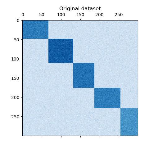
a_demo_of_the_spectral_co-clustering_algorithm
频谱共聚算法演示 翻译者:@N!no校验者:待校验 这个例子演示了如何使用谱协聚类算法生成数据集并对其进行双聚类处理。 数据集是使用 make_biclusters 函数生成的,该函数创建一个小值矩阵,并将大值植入双聚类。然后将行和列打乱并传递给光谱协聚算法。通过重新排列变换后的矩阵可以使双聚类连续,这展示出该算法找到双聚类的准确性。 1consensus score: 1.0 123456789101112131415161718192021222324252627282930313233343536373839404142print(__doc__)# Author: Kemal Eren <kemal@kemaleren.com># License: BSD 3 clauseimport numpy as npfrom matplotlib import pyplot as pltfrom sklearn.datasets import make_biclustersfrom sklearn.cluster import SpectralCoclus...

2020-09-26
whats_new_98_4_legend
0.98.4版本图例新特性创建图例并使用阴影和长方体对其进行调整。 1234567891011121314import matplotlib.pyplot as pltimport numpy as npax = plt.subplot(111)t1 = np.arange(0.0, 1.0, 0.01)for n in [1, 2, 3, 4]: plt.plot(t1, t1**n, label="n=%d"%(n,))leg = plt.legend(loc='best', ncol=2, mode="expand", shadow=True, fancybox=True)leg.get_frame().set_alpha(0.5)plt.show() 参考此示例显示了以下函数、方法、类和模块的使用: 12345import matplotlibmatplotlib.axes.Axes.legendmatplotlib.pyplot.legendmatplotlib.legend.Legendmatplo...
2020-10-24
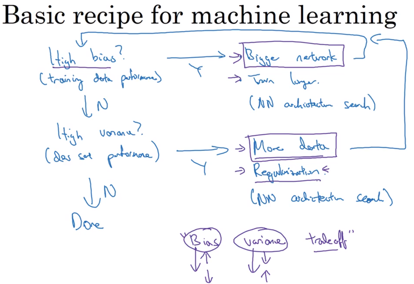
01深度学习的实用层面
# 深度学习的实用层面 > * [笔记模板](https://github.com/bighuang624/Andrew-Ng-Deep-Learning-notes) > * 相关的笔记都可以在github上先找到相关的笔记然后再修改,方便。 ## 数据划分:训练 / 验证 / 测试集 * 应用深度学习是一个典型的迭代过程。 * `->idea -> code -> employment->` * 对于一个需要解决的问题的样本数据,在建立模型的过程中,数据会被划分为以下几个部分: * 训练集(train set):用训练集对算法或模型进行**训练**过程; * 验证集(development set):利用验证集(又称为简单交叉验证集,hold-out cross validation set)进行**交叉验证**,**选择出最好的模型**; * 测试集(test set):最后利用测试集对模型进行测试,**获取模型运行的无偏估计**(对学习方法进行评估)。 * 在**小数据量**的时代,如 100、1000、10000 的数据量大小,可以将数据集...

2021-09-02
log
概述log 模块用于在程序中输出日志,它的使用十分简单,类似于fmt中的Print,一个最简单的示例如下: 1234567package mainimport "log"func main() { log.Print("Hello World")} 上面的程序会在命令行打印一条日志: 1>>> 2018/05/16 16:48:06 Hello World LoggerLogger是写入日志的基本组件,log模块中存在一个标准Logger,可以直接通过log进行访问,所以在上一节的例子中可以直接使用log.Print进行日志进行输出。但是在实际使用中,不同类型的日志可能拥有需求,仅标准Logger不能满足日志记录的需求,通过创建不同的Logger可以将不同类型的日志分类输出。使用logger前需要首先通过New函数创建一个Logger对象,函数声明如下: 1func New(out io.Writer, prefix string, flag int) *Logger 函数接收三个参数分别是日...

2020-09-26
boxplot_demo
箱形图用matplotlib可视化箱形图。 以下示例展示了如何使用Matplotlib可视化箱图。有许多选项可以控制它们的外观以及用于汇总数据的统计信息。 123456789101112131415161718192021222324252627282930313233343536373839404142434445464748495051525354555657585960616263import matplotlib.pyplot as pltimport numpy as npfrom matplotlib.patches import Polygon# Fixing random state for reproducibilitynp.random.seed(19680801)# fake up some dataspread = np.random.rand(50) * 100center = np.ones(25) * 50flier_high = np.random.rand(10) * 100 + 100flier_low = np.random.rand(10)...

2020-09-26
annotate_transform
注释变换此示例显示如何使用不同的坐标系进行注释。 有关注释功能的完整概述,另请参阅注释教程。 123456789101112131415161718192021222324252627282930313233import numpy as npimport matplotlib.pyplot as pltx = np.arange(0, 10, 0.005)y = np.exp(-x/2.) * np.sin(2*np.pi*x)fig, ax = plt.subplots()ax.plot(x, y)ax.set_xlim(0, 10)ax.set_ylim(-1, 1)xdata, ydata = 5, 0xdisplay, ydisplay = ax.transData.transform_point((xdata, ydata))bbox = dict(boxstyle="round", fc="0.8")arrowprops = dict( arrowstyle = "->", connect...


