
fill_between_alpha
在和Alpha之间填充
fill_between()函数在最小和最大边界之间生成阴影区域,这对于说明范围很有用。 它具有非常方便的用于将填充与逻辑范围组合的参数,例如,仅在某个阈值上填充曲线。
在最基本的层面上,fill_between 可用于增强图形的视觉外观。让我们将两个财务时间图与左边的简单线图和右边的实线进行比较。
1 | import matplotlib.pyplot as plt |

此处不需要Alpha通道,但它可以用于软化颜色以获得更具视觉吸引力的图形。在其他示例中,正如我们将在下面看到的,alpha通道在功能上非常有用,因为阴影区域可以重叠,alpha允许您查看两者。请注意,postscript格式不支持alpha(这是postscript限制,而不是matplotlib限制),因此在使用alpha时保存PNG,PDF或SVG中的数字。
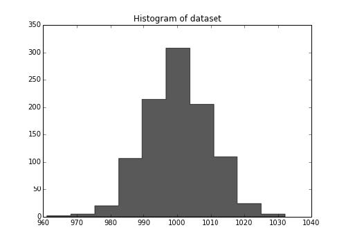
我们的下一个例子计算两个随机游走者群体,它们具有不同的正态分布的均值和标准差,从中得出步骤。我们使用共享区域绘制人口平均位置的+/-一个标准偏差。 这里的alpha通道非常有用,而不仅仅是审美。
1 | Nsteps, Nwalkers = 100, 250 |

where关键字参数非常便于突出显示图形的某些区域。其中布尔掩码的长度与x,ymin和ymax参数的长度相同,并且仅填充布尔掩码为True的区域。在下面的示例中,我们模拟单个随机游走者并计算人口位置的分析平均值和标准差。总体平均值显示为黑色虚线,并且与平均值的正/负一西格玛偏差显示为黄色填充区域。我们使用where掩码X> upper_bound来找到walker在一个sigma边界之上的区域,并将该区域遮蔽为蓝色。
1 | Nsteps = 500 |

填充区域的另一个方便用途是突出显示轴的水平或垂直跨度 - 因为matplotlib具有一些辅助函数 axhspan() 和axvspan() 以及示例axhspan Demo。
1 | plt.show() |
下载这个示例
本博客所有文章除特别声明外,均采用 CC BY-NC-SA 4.0 许可协议。转载请注明来源 Estom的博客!
相关推荐
2021-03-20
5 模型后处理
第五章 模型后处理 作者:Trent Hauck 译者:飞龙 协议:CC BY-NC-SA 4.0 5.1 K-fold 交叉验证这个秘籍中,我们会创建交叉验证,它可能是最重要的模型后处理验证练习。我们会在这个秘籍中讨论 k-fold 交叉验证。有几种交叉验证的种类,每个都有不同的随机化模式。K-fold 可能是一种最熟知的随机化模式。 准备我们会创建一些数据集,之后在不同的在不同的折叠上面训练分类器。值得注意的是,如果你可以保留一部分数据,那是最好的。例如,我们拥有N = 1000的数据集,如果我们保留 200 个数据点,之后使用其他 800 个数据点之间的交叉验证,来判断最佳参数。 工作原理首先,我们会创建一些伪造数据,之后测试参数,最后,我们会看看结果数据集的大小。 1234>>> N = 1000 >>> holdout = 200>>> from sklearn.datasets import make_regression >>> X, y = make_regression(1000...

2022-04-18
07 函数
函数是这样的一段 JavaScript 代码,它只定义一次,但可能被执行或调用多次。 简单来说,函数就是一组可重用的代码,你可以在你程序的任何地方调用他。 例如下述代码: 123function fn(){ console.log("this is function");} 函数定义定义函数有两种方式: 函数声明方式: 123function fn(){ console.log("this is function");} 字面量方式: 123var fun = fnction(){ console.log("this is function");} 函数调用定义一个函数并不会自动的执行它。定义了函数仅仅是赋予函数以名称并明确函数被调用时该做些什么。调用函数才会真正执行这些动作。 定义一个函数fn: 123function fn(){ console.log("this is function");} ...
2021-03-22
47 异步执行批量RPC处理
使用异步执行实现批量 RPC 处理 原文:https://pytorch.org/tutorials/intermediate/rpc_async_execution.html 作者:Shen Li 先决条件: PyTorch 分布式概述 分布式 RPC 框架入门 使用分布式 RPC 框架实现参数服务器 RPC 异步执行装饰器 本教程演示了如何使用@rpc.functions.async_execution装饰器来构建批量 RPC 应用,该装饰器通过减少阻止的 RPC 线程数和合并被调用方上的 CUDA 操作来帮助加快训练速度。 这使用 TorchServer 的相同想法进行批量推断。 注意 本教程需要 PyTorch v1.6.0 或更高版本。 基础知识先前的教程显示了使用torch.distributed.rpc构建分布式训练应用的步骤,但并未详细说明在处理 RPC 请求时被调用方发生的情况。 从 PyTorch v1.5 开始,每个 RPC 请求都会在被调用方上阻塞一个线程,以在该请求中执行该函数,直到该函数返回为止。 这适用于许多用例,但有一个警告。 如果用户函数例...

2021-03-22
44 分布式RPC框架
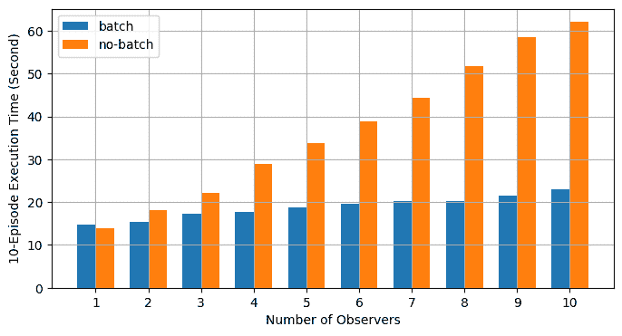
分布式 RPC 框架入门 原文:https://pytorch.org/tutorials/intermediate/rpc_tutorial.html 作者:Shen Li 先决条件: PyTorch 分布式概述 RPC API 文档 本教程使用两个简单的示例来演示如何使用torch.distributed.rpc包构建分布式训练,该包首先在 PyTorch v1.4 中作为原型功能引入。 这两个示例的源代码可以在 PyTorch 示例中找到。 先前的教程分布式数据并行入门和使用 PyTorch 编写分布式应用,描述了DistributedDataParallel,该模型支持特定的训练范例,该模型可在多个进程之间复制,每个进程都处理输入数据的拆分。 有时,您可能会遇到需要不同训练范例的场景。 例如: 在强化学习中,从环境中获取训练数据可能相对昂贵,而模型本身可能很小。 在这种情况下,产生多个并行运行的观察者并共享一个智能体可能会很有用。 在这种情况下,智能体将在本地负责训练,但是应用仍将需要库在观察者和训练者之间发送和接收数据。 您的模型可能太大,无法容纳在一台计算机上...
2021-03-20
34
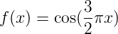
3.5. 验证曲线: 绘制分数以评估模型校验者: @正版乔 @正版乔 @小瑶翻译者: @Xi 每种估计器都有其优势和缺陷。它的泛化误差可以用偏差、方差和噪声来分解。估计值的 偏差 是不同训练集的平均误差。估计值的 方差 用来表示它对训练集的变化有多敏感。噪声是数据的一个属性。 在下面的图中,我们可以看到一个函数 和这个函数的一些噪声样本。 我们用三个不同的估计来拟合函数: 多项式特征为1,4和15的线性回归。我们看到,第一个估计最多只能为样本和真正的函数提供一个很差的拟合 ,因为它太简单了(高偏差),第二个估计几乎完全近似,最后一个估计完全接近训练数据, 但不能很好地拟合真实的函数,即对训练数据的变化(高方差)非常敏感。 偏差和方差是估计所固有的属性,我们通常必须选择合适的学习算法和超参数,以使得偏差和 方差都尽可能的低(参见偏差-方差困境)。 另一种降低方差的方法是使用更多的训练数据。不论如何,如果真实函数过于复杂并且不能用一个方 差较小的估计值来近似,则只能去收集更多的训练数据。 在一个简单的一维问题中,我们可以很容...

2021-03-20
32
3.3. 模型评估: 量化预测的质量校验者: @飓风 @小瑶 @FAME @v @Loopy翻译者: @小瑶 @片刻 @那伊抹微笑 有 3 种不同的 API 用于评估模型预测的质量: Estimator score method(估计器得分的方法): Estimators(估计器)有一个 score(得分) 方法,为其解决的问题提供了默认的 evaluation criterion (评估标准)。 在这个页面上没有相关讨论,但是在每个 estimator (估计器)的文档中会有相关的讨论。 Scoring parameter(评分参数): Model-evaluation tools (模型评估工具)使用 cross-validation (如 model_selection.cross_val_score 和 model_selection.GridSearchCV) 依靠 internal scoring strategy (内部 scoring(得分) 策略)。...


