
mathtext_examples
数学文本例子
Matplotlib的数学渲染引擎的选定功能。

Out:
1 | 0 $W^{3\beta}_{\delta_1 \rho_1 \sigma_2} = U^{3\beta}_{\delta_1 \rho_1} + \frac{1}{8 \pi 2} \int^{\alpha_2}_{\alpha_2} d \alpha^\prime_2 \left[\frac{ U^{2\beta}_{\delta_1 \rho_1} - \alpha^\prime_2U^{1\beta}_{\rho_1 \sigma_2} }{U^{0\beta}_{\rho_1 \sigma_2}}\right]$ |
1 | import matplotlib.pyplot as plt |
下载这个示例
本博客所有文章除特别声明外,均采用 CC BY-NC-SA 4.0 许可协议。转载请注明来源 Estom的博客!
相关推荐

2021-12-24
lsmod
lsmod显示已载入系统的模块 补充说明lsmod命令 用于显示已经加载到内核中的模块的状态信息。执行lsmod命令后会列出所有已载入系统的模块。Linux操作系统的核心具有模块化的特性,应此在编译核心时,务须把全部的功能都放入核心。您可以将这些功能编译成一个个单独的模块,待需要时再分别载入。 语法1lsmod 实例1234567891011121314151617181920212223242526272829303132333435363738394041424344454647484950515253545556575859606162636465666768697071727374[root@LinServ-1 ~]# lsmodModule Size Used byipv6 272801 15xfrm_nalgo 13381 1 ipv6crypto_api 12609 1 xfrm_nalgoip_conntrack_ftp 115...

2021-03-25
说明
参考文献 附加:sklearn分类的实验过程(以实战工程索引) cookbook入门教程(以流程索引) sklearn官方教程(以功能索引) sklearn API(以库名称索引) sklearn理解 按工作流程cookbook,数据加载、数据处理、分类、结果验证、模型使用 按官方文档doc,各种功能数据加载、特征选择、监督、无监督、评分 按api文档,各种类库
2021-04-08
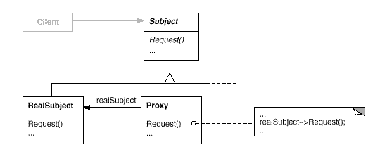
3.7 代理
代理模式1 概念别名 Surrogate 意图为其他对象提供一种代理以控制对这个对象的访问。 Provide a surrogate or placeholder for another object to control access to it. 结构按照使用场景代理有以下四类: 远程代理(Remote Proxy):控制对远程对象(不同地址空间)的访问,它负责将请求及其参数进行编码,并向不同地址空间中的对象发送已经编码的请求。 虚拟代理(Virtual Proxy):根据需要创建开销很大的对象,它可以缓存实体的附加信息,以便延迟对它的访问,例如在网站加载一个很大图片时,不能马上完成,可以用虚拟代理缓存图片的大小信息,然后生成一张临时图片代替原始图片。 保护代理(Protection Proxy):按权限控制对象的访问,它负责检查调用者是否具有实现一个请求所必须的访问权限。 智能代理(Smart Reference):取代了简单的指针,它在访问对象时执行一些附加操作:记录对象的引用次数;当第一次引用一个对象时,将它装入内存;在访问一个实际对象前,检查是否已经锁定了它,以确...

2021-03-09
现代软件工程——OO面向对象概述
面向对象技术 基本特征 **抽象:**抽象就是忽略一个主题中与当前目标无关的那些方面,以便更充分地注意与当前目标有关的方面。抽象并不打算了解全部问题,而只是选择其中的一部分,暂时不用部分细节。 封装:也就是把客观事物封装成抽象的类,并且类可以把自己的数据和方法只让可信的类或者对象操作,对不可信的进行信息隐藏。 继承:它可以使用现有类的所有功能,并在无需重新编写原来的类的情况下对这些功能进行扩展。 多态:多态性(polymorphisn)是允许你将父对象设置成为和一个或更多的他的子对象相等的技术,赋值之后,父对象就可以根据当前赋值给它的子对象的特性以不同的方式运作。简单的说,就是一句话:允许将子类类型的指针赋值给父类类型的指针。多态性是指允许不同类的对象对同一消息作出响应。 基本原则 单一职责原则:是指一个类的功能要单一,不能包罗万象。如同一个人一样,分配的工作不能太多,否则一天到晚虽然忙忙碌碌的,但效率却高不起来。 **开放封闭原则:**一个模块在扩展性方面应该是开放的而在更改性方面应该是封闭的。比如:一个网络模块,原来只服务端功能,而现在要加入客户端功能,那么应...
2021-03-31
7 高级表查询
系列七 高级的查询功能 分组查询group by 聚合函数avg 分组筛选having 结果排序order by 限制数量limit 123456789101112131415161718192021222324252627282930313233343536373839404142434445464748495051525354555657585960616263646566676869707172737475767778798081828384858687888990919293949596#第三十一课时--分组查询GROUP BY--按照用户所属省分进行分组SELECT * FROM cms_user GROUP BY proId;--按照字段位置进行分组SELECT * FROM cms_user GROUP BY 7;--按照多个字段进行分组SELECT F FROM cms_user GROUP BY sex,proId;--先写条件,后对满足条件的记录进行分组SELECT * FROM cms_user WHERE id > 5 GROUP BY sex...

2021-03-09
3 结构型设计模式
Structural Patterns(结构型模式)1 概述目标结构型模式涉及到如何组合类和对象以获得更大的结构。 结构型类模式采用继承机制来组合接口实现。 结构型对象模式不是对接口和实现进行组合,而是描述了如何对一些对象进行组合,从而实现新功能的一些方法。 因为可以在运行时改变对象组合关系,所以对象组合方式具有更大的灵活性,而这种机制用静态组合是不可能实现的。 Adapter(适配器) 将一个类的接口转换成客户希望的另外一个接口。 Adapter 模式使得原本由于接口不兼容而不能一起工作的那些类可以一起工作。 Bridge(桥接) 将抽象部分与它的实现部分分离,使它们都可以独立地变化。 Composite(组合) 将对象组合成树形结构以表示 “部分-整体” 的层次结构。 Composite 使得用户对于单个对象和组合对象的使用具有一致性。 Decorator(装饰) 动态地给一个对象添加一些额外的职责。 就增加功能来说,Decorator 模式相比生成子类更为灵活。 Facade(外观) 为子系统中的一组接口提供一个一致的界面。 Facade 模式定义了一个高...


