烹饪指南 本节列出了一些短小精悍 的 Pandas 实例与链接。
我们希望 Pandas 用户能积极踊跃地为本文档添加更多内容。为本节添加实用示例的链接或代码,是 Pandas 用户提交第一个 Pull Request 最好的选择。
本节列出了简单、精练、易上手的实例代码,以及 Stack Overflow 或 GitHub 上的链接,这些链接包含实例代码的更多详情。
pd 与 np 是 Pandas 与 Numpy 的缩写。为了让新手易于理解,其它模块是显式导入的。
下列实例均为 Python 3 代码,简单修改即可用于 Python 早期版本。
惯用语 以下是 Pandas 的惯用语。
对一列数据执行 if-then / if-then-else 操作,把计算结果赋值给一列或多列:
1
2
3
4
5
6
7
8
9
10
11
12
In [1 ]: df = pd.DataFrame({'AAA' : [4 , 5 , 6 , 7 ], ...: 'BBB' : [10 , 20 , 30 , 40 ], ...: 'CCC' : [100 , 50 , -30 , -50 ]}) ...: In [2 ]: df Out[2 ]: AAA BBB CCC 0 4 10 100 1 5 20 50 2 6 30 -30 3 7 40 -50
if-then… 在一列上执行 if-then 操作:
1
2
3
4
5
6
7
8
9
In [3 ]: df.loc[df.AAA >= 5 , 'BBB' ] = -1 In [4 ]: df Out[4 ]: AAA BBB CCC 0 4 10 100 1 5 -1 50 2 6 -1 -30 3 7 -1 -50
在两列上执行 if-then 操作:
1
2
3
4
5
6
7
8
9
In [5 ]: df.loc[df.AAA >= 5 , ['BBB' , 'CCC' ]] = 555 In [6 ]: df Out[6 ]: AAA BBB CCC 0 4 10 100 1 5 555 555 2 6 555 555 3 7 555 555
再添加一行代码,执行 -else 操作:
1
2
3
4
5
6
7
8
9
In [7 ]: df.loc[df.AAA < 5 , ['BBB' , 'CCC' ]] = 2000 In [8 ]: df Out[8 ]: AAA BBB CCC 0 4 2000 2000 1 5 555 555 2 6 555 555 3 7 555 555
或用 Pandas 的 where 设置掩码(mask):
1
2
3
4
5
6
7
8
9
10
11
12
In [9 ]: df_mask = pd.DataFrame({'AAA' : [True ] * 4 , ...: 'BBB' : [False ] * 4 , ...: 'CCC' : [True , False ] * 2 }) ...: In [10 ]: df.where(df_mask, -1000 ) Out[10 ]: AAA BBB CCC 0 4 -1000 2000 1 5 -1000 -1000 2 6 -1000 555 3 7 -1000 -1000
用 NumPy where() 函数实现 if-then-else
1
2
3
4
5
6
7
8
9
10
11
12
13
14
15
16
17
18
19
20
21
22
In [11 ]: df = pd.DataFrame({'AAA' : [4 , 5 , 6 , 7 ], ....: 'BBB' : [10 , 20 , 30 , 40 ], ....: 'CCC' : [100 , 50 , -30 , -50 ]}) ....: In [12 ]: df Out[12 ]: AAA BBB CCC 0 4 10 100 1 5 20 50 2 6 30 -30 3 7 40 -50 In [13 ]: df['logic' ] = np.where(df['AAA' ] > 5 , 'high' , 'low' ) In [14 ]: df Out[14 ]: AAA BBB CCC logic 0 4 10 100 low1 5 20 50 low2 6 30 -30 high3 7 40 -50 high
切割 用布尔条件切割 DataFrame
1
2
3
4
5
6
7
8
9
10
11
12
13
14
15
16
17
18
19
20
21
22
23
24
In [15 ]: df = pd.DataFrame({'AAA' : [4 , 5 , 6 , 7 ], ....: 'BBB' : [10 , 20 , 30 , 40 ], ....: 'CCC' : [100 , 50 , -30 , -50 ]}) ....: In [16 ]: df Out[16 ]: AAA BBB CCC 0 4 10 100 1 5 20 50 2 6 30 -30 3 7 40 -50 In [17 ]: df[df.AAA <= 5 ] Out[17 ]: AAA BBB CCC 0 4 10 100 1 5 20 50 In [18 ]: df[df.AAA > 5 ] Out[18 ]: AAA BBB CCC 2 6 30 -30 3 7 40 -50
设置条件 多列条件选择
1
2
3
4
5
6
7
8
9
10
11
12
In [19 ]: df = pd.DataFrame({'AAA' : [4 , 5 , 6 , 7 ], ....: 'BBB' : [10 , 20 , 30 , 40 ], ....: 'CCC' : [100 , 50 , -30 , -50 ]}) ....: In [20 ]: df Out[20 ]: AAA BBB CCC 0 4 10 100 1 5 20 50 2 6 30 -30 3 7 40 -50
和(&),不赋值,直接返回 Series:
1
2
3
4
5
In [21 ]: df.loc[(df['BBB' ] < 25 ) & (df['CCC' ] >= -40 ), 'AAA' ] Out[21 ]: 0 4 1 5 Name: AAA, dtype: int64
或(|),不赋值,直接返回 Series:
1
2
3
4
5
6
7
In [22 ]: df.loc[(df['BBB' ] > 25 ) | (df['CCC' ] >= -40 ), 'AAA' ] Out[22 ]: 0 4 1 5 2 6 3 7 Name: AAA, dtype: int64
或(|),赋值,修改 DataFrame:
1
2
3
4
5
6
7
8
9
In [23 ]: df.loc[(df['BBB' ] > 25 ) | (df['CCC' ] >= 75 ), 'AAA' ] = 0.1 In [24 ]: df Out[24 ]: AAA BBB CCC 0 0.1 10 100 1 5.0 20 50 2 0.1 30 -30 3 0.1 40 -50
用 argsort 选择最接近指定值的行
1
2
3
4
5
6
7
8
9
10
11
12
13
14
15
16
17
18
19
20
21
22
In [25 ]: df = pd.DataFrame({'AAA' : [4 , 5 , 6 , 7 ], ....: 'BBB' : [10 , 20 , 30 , 40 ], ....: 'CCC' : [100 , 50 , -30 , -50 ]}) ....: In [26 ]: df Out[26 ]: AAA BBB CCC 0 4 10 100 1 5 20 50 2 6 30 -30 3 7 40 -50 In [27 ]: aValue = 43.0 In [28 ]: df.loc[(df.CCC - aValue).abs ().argsort()] Out[28 ]: AAA BBB CCC 1 5 20 50 0 4 10 100 2 6 30 -30 3 7 40 -50
用二进制运算符动态减少条件列表
1
2
3
4
5
6
7
8
9
10
11
12
13
14
15
16
17
18
In [29 ]: df = pd.DataFrame({'AAA' : [4 , 5 , 6 , 7 ], ....: 'BBB' : [10 , 20 , 30 , 40 ], ....: 'CCC' : [100 , 50 , -30 , -50 ]}) ....: In [30 ]: df Out[30 ]: AAA BBB CCC 0 4 10 100 1 5 20 50 2 6 30 -30 3 7 40 -50 In [31 ]: Crit1 = df.AAA <= 5.5 In [32 ]: Crit2 = df.BBB == 10.0 In [33 ]: Crit3 = df.CCC > -40.0
硬编码方式为:
1 In [34 ]: AllCrit = Crit1 & Crit2 & Crit3
生成动态条件列表:
1
2
3
4
5
6
7
8
9
10
In [35 ]: import functools In [36 ]: CritList = [Crit1, Crit2, Crit3] In [37 ]: AllCrit = functools.reduce(lambda x, y: x & y, CritList) In [38 ]: df[AllCrit] Out[38 ]: AAA BBB CCC 0 4 10 100
选择 DataFrames 更多信息,请参阅索引 文档。
行标签与值作为条件
1
2
3
4
5
6
7
8
9
10
11
12
13
14
15
16
17
18
In [39 ]: df = pd.DataFrame({'AAA' : [4 , 5 , 6 , 7 ], ....: 'BBB' : [10 , 20 , 30 , 40 ], ....: 'CCC' : [100 , 50 , -30 , -50 ]}) ....: In [40 ]: df Out[40 ]: AAA BBB CCC 0 4 10 100 1 5 20 50 2 6 30 -30 3 7 40 -50 In [41 ]: df[(df.AAA <= 6 ) & (df.index.isin([0 , 2 , 4 ]))] Out[41 ]: AAA BBB CCC 0 4 10 100 2 6 30 -30
标签切片用 loc,位置切片用 iloc
1
2
3
4
5
In [42 ]: df = pd.DataFrame({'AAA' : [4 , 5 , 6 , 7 ], ....: 'BBB' : [10 , 20 , 30 , 40 ], ....: 'CCC' : [100 , 50 , -30 , -50 ]}, ....: index=['foo' , 'bar' , 'boo' , 'kar' ]) ....:
前 2 个是显式切片方法,第 3 个是通用方法:
位置切片,Python 切片风格,不包括结尾数据;
标签切片,非 Python 切片风格,包括结尾数据;
通用切片,支持两种切片风格,取决于切片用的是标签还是位置。
1
2
3
4
5
6
7
8
9
10
11
12
13
14
15
16
17
18
19
20
21
In [43 ]: df.loc['bar' :'kar' ] Out[43 ]: AAA BBB CCC bar 5 20 50 boo 6 30 -30 kar 7 40 -50 In [44 ]: df.iloc[0 :3 ] Out[44 ]: AAA BBB CCC foo 4 10 100 bar 5 20 50 boo 6 30 -30 In [45 ]: df.loc['bar' :'kar' ] Out[45 ]: AAA BBB CCC bar 5 20 50 boo 6 30 -30 kar 7 40 -50
包含整数,且不从 0 开始的索引,或不是逐步递增的索引会引发歧义。
1
2
3
4
5
6
7
8
9
10
11
12
13
14
15
16
17
18
19
In [46 ]: data = {'AAA' : [4 , 5 , 6 , 7 ], ....: 'BBB' : [10 , 20 , 30 , 40 ], ....: 'CCC' : [100 , 50 , -30 , -50 ]} ....: In [47 ]: df2 = pd.DataFrame(data=data, index=[1 , 2 , 3 , 4 ]) In [48 ]: df2.iloc[1 :3 ] Out[48 ]: AAA BBB CCC 2 5 20 50 3 6 30 -30 In [49 ]: df2.loc[1 :3 ] Out[49 ]: AAA BBB CCC 1 4 10 100 2 5 20 50 3 6 30 -30
用逆运算符 (~)提取掩码的反向内容
1
2
3
4
5
6
7
8
9
10
11
12
13
14
15
16
17
18
In [50 ]: df = pd.DataFrame({'AAA' : [4 , 5 , 6 , 7 ], ....: 'BBB' : [10 , 20 , 30 , 40 ], ....: 'CCC' : [100 , 50 , -30 , -50 ]}) ....: In [51 ]: df Out[51 ]: AAA BBB CCC 0 4 10 100 1 5 20 50 2 6 30 -30 3 7 40 -50 In [52 ]: df[~((df.AAA <= 6 ) & (df.index.isin([0 , 2 , 4 ])))] Out[52 ]: AAA BBB CCC 1 5 20 50 3 7 40 -50
生成新列 用 applymap 高效动态生成新列
1
2
3
4
5
6
7
8
9
10
11
12
13
14
15
16
17
18
19
20
21
22
23
24
25
26
27
28
In [53 ]: df = pd.DataFrame({'AAA' : [1 , 2 , 1 , 3 ], ....: 'BBB' : [1 , 1 , 2 , 2 ], ....: 'CCC' : [2 , 1 , 3 , 1 ]}) ....: In [54 ]: df Out[54 ]: AAA BBB CCC 0 1 1 2 1 2 1 1 2 1 2 3 3 3 2 1 In [55 ]: source_cols = df.columns In [56 ]: new_cols = [str (x) + "_cat" for x in source_cols] In [57 ]: categories = {1 : 'Alpha' , 2 : 'Beta' , 3 : 'Charlie' } In [58 ]: df[new_cols] = df[source_cols].applymap(categories.get) In [59 ]: df Out[59 ]: AAA BBB CCC AAA_cat BBB_cat CCC_cat 0 1 1 2 Alpha Alpha Beta1 2 1 1 Beta Alpha Alpha2 1 2 3 Alpha Beta Charlie3 3 2 1 Charlie Beta Alpha
分组时用 min()
1
2
3
4
5
6
7
8
9
10
11
12
13
14
15
In [60 ]: df = pd.DataFrame({'AAA' : [1 , 1 , 1 , 2 , 2 , 2 , 3 , 3 ], ....: 'BBB' : [2 , 1 , 3 , 4 , 5 , 1 , 2 , 3 ]}) ....: In [61 ]: df Out[61 ]: AAA BBB 0 1 2 1 1 1 2 1 3 3 2 4 4 2 5 5 2 1 6 3 2 7 3 3
方法1:用 idxmin() 提取每组最小值的索引
1
2
3
4
5
6
In [62 ]: df.loc[df.groupby("AAA" )["BBB" ].idxmin()] Out[62 ]: AAA BBB 1 1 1 5 2 1 6 3 2
方法 2:先排序,再提取每组的第一个值
1
2
3
4
5
6
In [63 ]: df.sort_values(by="BBB" ).groupby("AAA" , as_index=False ).first() Out[63 ]: AAA BBB 0 1 1 1 2 1 2 3 2
注意,提取的数据一样,但索引不一样。
多层索引 更多信息,请参阅多层索引 文档。
用带标签的字典创建多层索引
1
2
3
4
5
6
7
8
9
10
11
12
13
14
15
16
17
18
19
20
21
22
23
24
25
26
27
28
29
30
31
32
33
34
35
36
37
38
39
40
41
42
43
44
45
46
47
48
49
50
51
52
53
54
55
56
57
58
59
60
61
62
63
64
65
66
67
In [64 ]: df = pd.DataFrame({'row' : [0 , 1 , 2 ], ....: 'One_X' : [1.1 , 1.1 , 1.1 ], ....: 'One_Y' : [1.2 , 1.2 , 1.2 ], ....: 'Two_X' : [1.11 , 1.11 , 1.11 ], ....: 'Two_Y' : [1.22 , 1.22 , 1.22 ]}) ....: In [65 ]: df Out[65 ]: row One_X One_Y Two_X Two_Y 0 0 1.1 1.2 1.11 1.22 1 1 1.1 1.2 1.11 1.22 2 2 1.1 1.2 1.11 1.22 In [66 ]: df = df.set_index('row' ) In [67 ]: df Out[67 ]: One_X One_Y Two_X Two_Y row 0 1.1 1.2 1.11 1.22 1 1.1 1.2 1.11 1.22 2 1.1 1.2 1.11 1.22 In [68 ]: df.columns = pd.MultiIndex.from_tuples([tuple (c.split('_' )) ....: for c in df.columns]) ....: In [69 ]: df Out[69 ]: One Two X Y X Y row 0 1.1 1.2 1.11 1.22 1 1.1 1.2 1.11 1.22 2 1.1 1.2 1.11 1.22 In [70 ]: df = df.stack(0 ).reset_index(1 ) In [71 ]: df Out[71 ]: level_1 X Y row 0 One 1.10 1.20 0 Two 1.11 1.22 1 One 1.10 1.20 1 Two 1.11 1.22 2 One 1.10 1.20 2 Two 1.11 1.22 In [72 ]: df.columns = ['Sample' , 'All_X' , 'All_Y' ] In [73 ]: df Out[73 ]: Sample All_X All_Y row 0 One 1.10 1.20 0 Two 1.11 1.22 1 One 1.10 1.20 1 Two 1.11 1.22 2 One 1.10 1.20 2 Two 1.11 1.22
运算 多层索引运算要用广播机制
1
2
3
4
5
6
7
8
9
10
11
12
13
14
15
16
17
18
19
20
21
In [74 ]: cols = pd.MultiIndex.from_tuples([(x, y) for x in ['A' , 'B' , 'C' ] ....: for y in ['O' , 'I' ]]) ....: In [75 ]: df = pd.DataFrame(np.random.randn(2 , 6 ), index=['n' , 'm' ], columns=cols) In [76 ]: df Out[76 ]: A B C O I O I O I n 0.469112 -0.282863 -1.509059 -1.135632 1.212112 -0.173215 m 0.119209 -1.044236 -0.861849 -2.104569 -0.494929 1.071804 In [77 ]: df = df.div(df['C' ], level=1 ) In [78 ]: df Out[78 ]: A B C O I O I O I n 0.387021 1.633022 -1.244983 6.556214 1.0 1.0 m -0.240860 -0.974279 1.741358 -1.963577 1.0 1.0
切片 用 xs 切片多层索引
1
2
3
4
5
6
7
8
9
10
11
12
13
14
15
16
In [79 ]: coords = [('AA' , 'one' ), ('AA' , 'six' ), ('BB' , 'one' ), ('BB' , 'two' ), ....: ('BB' , 'six' )] ....: In [80 ]: index = pd.MultiIndex.from_tuples(coords) In [81 ]: df = pd.DataFrame([11 , 22 , 33 , 44 , 55 ], index, ['MyData' ]) In [82 ]: df Out[82 ]: MyData AA one 11 six 22 BB one 33 two 44 six 55
提取第一层与索引第一个轴的交叉数据:
1 2 3 4 5 6 7 In [83 ]: df.xs('BB' , level=0 , axis=0 ) Out[83 ]: MyData one 33 two 44 six 55
……现在是第 1 个轴的第 2 层
1
2
3
4
5
In [84 ]: df.xs('six' , level=1 , axis=0 ) Out[84 ]: MyData AA 22 BB 55
用 xs 切片多层索引,方法 #2
1
2
3
4
5
6
7
8
9
10
11
12
13
14
15
16
17
18
19
20
21
22
23
24
25
26
27
28
29
30
31
32
33
34
35
36
37
38
39
40
41
42
43
44
45
46
47
48
49
50
51
52
53
54
55
56
57
58
59
60
61
62
63
64
65
66
67
68
69
70
71
72
73
74
75
In [85 ]: import itertools In [86 ]: index = list (itertools.product(['Ada' , 'Quinn' , 'Violet' ], ....: ['Comp' , 'Math' , 'Sci' ])) ....: In [87 ]: headr = list (itertools.product(['Exams' , 'Labs' ], ['I' , 'II' ])) In [88 ]: indx = pd.MultiIndex.from_tuples(index, names=['Student' , 'Course' ]) In [89 ]: cols = pd.MultiIndex.from_tuples(headr) In [90 ]: data = [[70 + x + y + (x * y) % 3 for x in range (4 )] for y in range (9 )] In [91 ]: df = pd.DataFrame(data, indx, cols) In [92 ]: df Out[92 ]: Exams Labs I II I II Student Course Ada Comp 70 71 72 73 Math 71 73 75 74 Sci 72 75 75 75 Quinn Comp 73 74 75 76 Math 74 76 78 77 Sci 75 78 78 78 Violet Comp 76 77 78 79 Math 77 79 81 80 Sci 78 81 81 81 In [93 ]: All = slice (None ) In [94 ]: df.loc['Violet' ] Out[94 ]: Exams Labs I II I II Course Comp 76 77 78 79 Math 77 79 81 80 Sci 78 81 81 81 In [95 ]: df.loc[(All, 'Math' ), All] Out[95 ]: Exams Labs I II I II Student Course Ada Math 71 73 75 74 Quinn Math 74 76 78 77 Violet Math 77 79 81 80 In [96 ]: df.loc[(slice ('Ada' , 'Quinn' ), 'Math' ), All] Out[96 ]: Exams Labs I II I II Student Course Ada Math 71 73 75 74 Quinn Math 74 76 78 77 In [97 ]: df.loc[(All, 'Math' ), ('Exams' )] Out[97 ]: I II Student Course Ada Math 71 73 Quinn Math 74 76 Violet Math 77 79 In [98 ]: df.loc[(All, 'Math' ), (All, 'II' )] Out[98 ]: Exams Labs II II Student Course Ada Math 73 74 Quinn Math 76 77 Violet Math 79 80
用 xs 设置多层索引比例
排序 用多层索引按指定列或列序列表排序x
1
2
3
4
5
6
7
8
9
10
11
12
13
14
In [99 ]: df.sort_values(by=('Labs' , 'II' ), ascending=False ) Out[99 ]: Exams Labs I II I II Student Course Violet Sci 78 81 81 81 Math 77 79 81 80 Comp 76 77 78 79 Quinn Sci 75 78 78 78 Math 74 76 78 77 Comp 73 74 75 76 Ada Sci 72 75 75 75 Math 71 73 75 74 Comp 70 71 72 73
部分选择,需要排序
层级 为多层索引添加一层
平铺结构化列
缺失数据 缺失数据 文档。
向前填充逆序时间序列。
1
2
3
4
5
6
7
8
9
10
11
12
13
14
15
16
17
18
19
20
21
22
23
24
25
26
In [100 ]: df = pd.DataFrame(np.random.randn(6 , 1 ), .....: index=pd.date_range('2013-08-01' , periods=6 , freq='B' ), .....: columns=list ('A' )) .....: In [101 ]: df.loc[df.index[3 ], 'A' ] = np.nan In [102 ]: df Out[102 ]: A 2013 -08-01 0.721555 2013 -08-02 -0.706771 2013 -08-05 -1.039575 2013 -08-06 NaN2013 -08-07 -0.424972 2013 -08-08 0.567020 In [103 ]: df.reindex(df.index[::-1 ]).ffill() Out[103 ]: A 2013 -08-08 0.567020 2013 -08-07 -0.424972 2013 -08-06 -0.424972 2013 -08-05 -1.039575 2013 -08-02 -0.706771 2013 -08-01 0.721555
空值时重置为 0,有值时累加
替换 用反引用替换
分组 分组 文档。
用 apply 执行分组基础操作
与聚合不同,传递给 DataFrame 子集的 apply 可回调,可以访问所有列。
1
2
3
4
5
6
7
8
9
10
11
12
13
14
15
16
17
18
19
20
21
22
23
24
25
In [104 ]: df = pd.DataFrame({'animal' : 'cat dog cat fish dog cat cat' .split(), .....: 'size' : list ('SSMMMLL' ), .....: 'weight' : [8 , 10 , 11 , 1 , 20 , 12 , 12 ], .....: 'adult' : [False ] * 5 + [True ] * 2 }) .....: In [105 ]: df Out[105 ]: animal size weight adult 0 cat S 8 False 1 dog S 10 False 2 cat M 11 False 3 fish M 1 False 4 dog M 20 False 5 cat L 12 True 6 cat L 12 True In [106 ]: df.groupby('animal' ).apply(lambda subf: subf['size' ][subf['weight' ].idxmax()]) Out[106 ]: animal cat L dog M fish M dtype: object
使用 get_group
1
2
3
4
5
6
7
8
9
In [107 ]: gb = df.groupby(['animal' ]) In [108 ]: gb.get_group('cat' ) Out[108 ]: animal size weight adult 0 cat S 8 False 2 cat M 11 False 5 cat L 12 True 6 cat L 12 True
为同一分组的不同内容使用 Apply 函数
1
2
3
4
5
6
7
8
9
10
11
12
13
14
15
16
17
18
In [109 ]: def GrowUp (x ): .....: avg_weight = sum (x[x['size' ] == 'S' ].weight * 1.5 ) .....: avg_weight += sum (x[x['size' ] == 'M' ].weight * 1.25 ) .....: avg_weight += sum (x[x['size' ] == 'L' ].weight) .....: avg_weight /= len (x) .....: return pd.Series(['L' , avg_weight, True ], .....: index=['size' , 'weight' , 'adult' ]) .....: In [110 ]: expected_df = gb.apply(GrowUp) In [111 ]: expected_df Out[111 ]: size weight adult animal cat L 12.4375 True dog L 20.0000 True fish L 1.2500 True
Apply 函数扩展
1
2
3
4
5
6
7
8
9
10
11
12
13
14
15
16
17
18
19
20
21
22
23
In [112 ]: S = pd.Series([i / 100.0 for i in range (1 , 11 )]) In [113 ]: def cum_ret (x, y ): .....: return x * (1 + y) .....: In [114 ]: def red (x ): .....: return functools.reduce(cum_ret, x, 1.0 ) .....: In [115 ]: S.expanding().apply(red, raw=True ) Out[115 ]: 0 1.010000 1 1.030200 2 1.061106 3 1.103550 4 1.158728 5 1.228251 6 1.314229 7 1.419367 8 1.547110 9 1.701821 dtype: float64
用分组里的剩余值的平均值进行替换
1
2
3
4
5
6
7
8
9
10
11
12
13
14
15
16
In [116 ]: df = pd.DataFrame({'A' : [1 , 1 , 2 , 2 ], 'B' : [1 , -1 , 1 , 2 ]}) In [117 ]: gb = df.groupby('A' ) In [118 ]: def replace (g ): .....: mask = g < 0 .....: return g.where(mask, g[~mask].mean()) .....: In [119 ]: gb.transform(replace) Out[119 ]: B 0 1.0 1 -1.0 2 1.5 3 1.5
按聚合数据排序
1
2
3
4
5
6
7
8
9
10
11
12
13
14
15
16
17
18
19
20
In [120 ]: df = pd.DataFrame({'code' : ['foo' , 'bar' , 'baz' ] * 2 , .....: 'data' : [0.16 , -0.21 , 0.33 , 0.45 , -0.59 , 0.62 ], .....: 'flag' : [False , True ] * 3 }) .....: In [121 ]: code_groups = df.groupby('code' ) In [122 ]: agg_n_sort_order = code_groups[['data' ]].transform(sum ).sort_values(by='data' ) In [123 ]: sorted_df = df.loc[agg_n_sort_order.index] In [124 ]: sorted_df Out[124 ]: code data flag 1 bar -0.21 True 4 bar -0.59 False 0 foo 0.16 False 3 foo 0.45 True 2 baz 0.33 False 5 baz 0.62 True
创建多个聚合列
1
2
3
4
5
6
7
8
9
10
11
12
13
14
15
16
17
18
19
20
21
22
23
24
25
26
27
28
29
30
31
32
33
34
35
36
37
38
39
40
41
In [125 ]: rng = pd.date_range(start="2014-10-07" , periods=10 , freq='2min' ) In [126 ]: ts = pd.Series(data=list (range (10 )), index=rng) In [127 ]: def MyCust (x ): .....: if len (x) > 2 : .....: return x[1 ] * 1.234 .....: return pd.NaT .....: In [128 ]: mhc = {'Mean' : np.mean, 'Max' : np.max , 'Custom' : MyCust} In [129 ]: ts.resample("5min" ).apply(mhc) Out[129 ]: Mean 2014 -10 -07 00 :00 :00 1 2014 -10 -07 00 :05:00 3.5 2014 -10 -07 00 :10 :00 6 2014 -10 -07 00 :15 :00 8.5 Max 2014 -10 -07 00 :00 :00 2 2014 -10 -07 00 :05:00 4 2014 -10 -07 00 :10 :00 7 2014 -10 -07 00 :15 :00 9 Custom 2014 -10 -07 00 :00 :00 1.234 2014 -10 -07 00 :05:00 NaT 2014 -10 -07 00 :10 :00 7.404 2014 -10 -07 00 :15 :00 NaT dtype: object In [130 ]: ts Out[130 ]: 2014 -10 -07 00 :00 :00 0 2014 -10 -07 00 :02:00 1 2014 -10 -07 00 :04:00 2 2014 -10 -07 00 :06:00 3 2014 -10 -07 00 :08:00 4 2014 -10 -07 00 :10 :00 5 2014 -10 -07 00 :12 :00 6 2014 -10 -07 00 :14 :00 7 2014 -10 -07 00 :16 :00 8 2014 -10 -07 00 :18 :00 9 Freq: 2T, dtype: int64
为 DataFrame 创建值计数列
1
2
3
4
5
6
7
8
9
10
11
12
13
14
15
16
17
18
19
20
21
In [131 ]: df = pd.DataFrame({'Color' : 'Red Red Red Blue' .split(), .....: 'Value' : [100 , 150 , 50 , 50 ]}) .....: In [132 ]: df Out[132 ]: Color Value 0 Red 100 1 Red 150 2 Red 50 3 Blue 50 In [133 ]: df['Counts' ] = df.groupby(['Color' ]).transform(len ) In [134 ]: df Out[134 ]: Color Value Counts 0 Red 100 3 1 Red 150 3 2 Red 50 3 3 Blue 50 1
基于索引唯一某列不同分组的值
1
2
3
4
5
6
7
8
9
10
11
12
13
14
15
16
17
18
19
20
21
22
23
24
25
26
27
28
In [135 ]: df = pd.DataFrame({'line_race' : [10 , 10 , 8 , 10 , 10 , 8 ], .....: 'beyer' : [99 , 102 , 103 , 103 , 88 , 100 ]}, .....: index=['Last Gunfighter' , 'Last Gunfighter' , .....: 'Last Gunfighter' , 'Paynter' , 'Paynter' , .....: 'Paynter' ]) .....: In [136 ]: df Out[136 ]: line_race beyer Last Gunfighter 10 99 Last Gunfighter 10 102 Last Gunfighter 8 103 Paynter 10 103 Paynter 10 88 Paynter 8 100 In [137 ]: df['beyer_shifted' ] = df.groupby(level=0 )['beyer' ].shift(1 ) In [138 ]: df Out[138 ]: line_race beyer beyer_shifted Last Gunfighter 10 99 NaN Last Gunfighter 10 102 99.0 Last Gunfighter 8 103 102.0 Paynter 10 103 NaN Paynter 10 88 103.0 Paynter 8 100 88.0
选择每组最大值的行
1
2
3
4
5
6
7
8
9
10
11
12
13
14
15
In [139 ]: df = pd.DataFrame({'host' : ['other' , 'other' , 'that' , 'this' , 'this' ], .....: 'service' : ['mail' , 'web' , 'mail' , 'mail' , 'web' ], .....: 'no' : [1 , 2 , 1 , 2 , 1 ]}).set_index(['host' , 'service' ]) .....: In [140 ]: mask = df.groupby(level=0 ).agg('idxmax' ) In [141 ]: df_count = df.loc[mask['no' ]].reset_index() In [142 ]: df_count Out[142 ]: host service no 0 other web 2 1 that mail 1 2 this mail 2
Python itertools.groupby 式分组
1
2
3
4
5
6
7
8
9
10
11
12
13
14
15
16
17
18
19
20
21
22
23
In [143 ]: df = pd.DataFrame([0 , 1 , 0 , 1 , 1 , 1 , 0 , 1 , 1 ], columns=['A' ]) In [144 ]: df.A.groupby((df.A != df.A.shift()).cumsum()).groups Out[144 ]: {1 : Int64Index([0 ], dtype='int64' ), 2 : Int64Index([1 ], dtype='int64' ), 3 : Int64Index([2 ], dtype='int64' ), 4 : Int64Index([3 , 4 , 5 ], dtype='int64' ), 5 : Int64Index([6 ], dtype='int64' ), 6 : Int64Index([7 , 8 ], dtype='int64' )} In [145 ]: df.A.groupby((df.A != df.A.shift()).cumsum()).cumsum() Out[145 ]: 0 0 1 1 2 0 3 1 4 2 5 3 6 0 7 1 8 2 Name: A, dtype: int64
扩展数据 Alignment and to-date
基于计数值进行移动窗口计算
按时间间隔计算滚动平均
分割 分割 DataFrame
按指定逻辑,将不同的行,分割成 DataFrame 列表。
1
2
3
4
5
6
7
8
9
10
11
12
13
14
15
16
17
18
19
20
21
22
23
24
25
26
27
28
29
In [146 ]: df = pd.DataFrame(data={'Case' : ['A' , 'A' , 'A' , 'B' , 'A' , 'A' , 'B' , 'A' , .....: 'A' ], .....: 'Data' : np.random.randn(9 )}) .....: In [147 ]: dfs = list (zip (*df.groupby((1 * (df['Case' ] == 'B' )).cumsum() .....: .rolling(window=3 , min_periods=1 ).median())))[-1 ] .....: In [148 ]: dfs[0 ] Out[148 ]: Case Data 0 A 0.276232 1 A -1.087401 2 A -0.673690 3 B 0.113648 In [149 ]: dfs[1 ] Out[149 ]: Case Data 4 A -1.478427 5 A 0.524988 6 B 0.404705 In [150 ]: dfs[2 ] Out[150 ]: Case Data 7 A 0.577046 8 A -1.715002
透视表 透视表 文档。
部分汇总与小计
1
2
3
4
5
6
7
8
9
10
11
12
13
14
15
16
17
18
19
20
21
22
23
24
25
26
27
28
In [151 ]: df = pd.DataFrame(data={'Province' : ['ON' , 'QC' , 'BC' , 'AL' , 'AL' , 'MN' , 'ON' ], .....: 'City' : ['Toronto' , 'Montreal' , 'Vancouver' , .....: 'Calgary' , 'Edmonton' , 'Winnipeg' , .....: 'Windsor' ], .....: 'Sales' : [13 , 6 , 16 , 8 , 4 , 3 , 1 ]}) .....: In [152 ]: table = pd.pivot_table(df, values=['Sales' ], index=['Province' ], .....: columns=['City' ], aggfunc=np.sum , margins=True ) .....: In [153 ]: table.stack('City' ) Out[153 ]: Sales Province City AL All 12.0 Calgary 8.0 Edmonton 4.0 BC All 16.0 Vancouver 16.0 ... ...All Montreal 6.0 Toronto 13.0 Vancouver 16.0 Windsor 1.0 Winnipeg 3.0 [20 rows x 1 columns]
类似 R 的 plyr 频率表
1
2
3
4
5
6
7
8
9
10
11
12
13
14
15
16
17
18
19
20
21
22
23
24
25
26
27
28
29
In [154 ]: grades = [48 , 99 , 75 , 80 , 42 , 80 , 72 , 68 , 36 , 78 ] In [155 ]: df = pd.DataFrame({'ID' : ["x%d" % r for r in range (10 )], .....: 'Gender' : ['F' , 'M' , 'F' , 'M' , 'F' , .....: 'M' , 'F' , 'M' , 'M' , 'M' ], .....: 'ExamYear' : ['2007' , '2007' , '2007' , '2008' , '2008' , .....: '2008' , '2008' , '2009' , '2009' , '2009' ], .....: 'Class' : ['algebra' , 'stats' , 'bio' , 'algebra' , .....: 'algebra' , 'stats' , 'stats' , 'algebra' , .....: 'bio' , 'bio' ], .....: 'Participated' : ['yes' , 'yes' , 'yes' , 'yes' , 'no' , .....: 'yes' , 'yes' , 'yes' , 'yes' , 'yes' ], .....: 'Passed' : ['yes' if x > 50 else 'no' for x in grades], .....: 'Employed' : [True , True , True , False , .....: False , False , False , True , True , False ], .....: 'Grade' : grades}) .....: In [156 ]: df.groupby('ExamYear' ).agg({'Participated' : lambda x: x.value_counts()['yes' ], .....: 'Passed' : lambda x: sum (x == 'yes' ), .....: 'Employed' : lambda x: sum (x), .....: 'Grade' : lambda x: sum (x) / len (x)}) .....: Out[156 ]: Participated Passed Employed Grade ExamYear 2007 3 2 3 74.000000 2008 3 3 0 68.500000 2009 3 2 2 60.666667
按年生成 DataFrame
跨列表创建年月:
1
2
3
4
5
6
7
8
9
10
11
12
13
14
15
16
17
18
19
20
21
In [157 ]: df = pd.DataFrame({'value' : np.random.randn(36 )}, .....: index=pd.date_range('2011-01-01' , freq='M' , periods=36 )) .....: In [158 ]: pd.pivot_table(df, index=df.index.month, columns=df.index.year, .....: values='value' , aggfunc='sum' ) .....: Out[158 ]: 2011 2012 2013 1 -1.039268 -0.968914 2.565646 2 -0.370647 -1.294524 1.431256 3 -1.157892 0.413738 1.340309 4 -1.344312 0.276662 -1.170299 5 0.844885 -0.472035 -0.226169 6 1.075770 -0.013960 0.410835 7 -0.109050 -0.362543 0.813850 8 1.643563 -0.006154 0.132003 9 -1.469388 -0.923061 -0.827317 10 0.357021 0.895717 -0.076467 11 -0.674600 0.805244 -1.187678 12 -1.776904 -1.206412 1.130127
Apply 函数 把嵌入列表转换为多层索引 DataFrame
1
2
3
4
5
6
7
8
9
10
11
12
13
14
15
16
17
18
19
20
21
22
In [159 ]: df = pd.DataFrame(data={'A' : [[2 , 4 , 8 , 16 ], [100 , 200 ], [10 , 20 , 30 ]], .....: 'B' : [['a' , 'b' , 'c' ], ['jj' , 'kk' ], ['ccc' ]]}, .....: index=['I' , 'II' , 'III' ]) .....: In [160 ]: def SeriesFromSubList (aList ): .....: return pd.Series(aList) .....: In [161 ]: df_orgz = pd.concat({ind: row.apply(SeriesFromSubList) .....: for ind, row in df.iterrows()}) .....: In [162 ]: df_orgz Out[162 ]: 0 1 2 3 I A 2 4 8 16.0 B a b c NaN II A 100 200 NaN NaN B jj kk NaN NaN III A 10 20 30 NaN B ccc NaN NaN NaN
返回 Series
Rolling Apply to multiple columns where function calculates a Series before a Scalar from the Series is returned
1
2
3
4
5
6
7
8
9
10
11
12
13
14
15
16
17
18
19
20
21
22
23
24
25
26
27
28
29
30
31
32
33
34
35
36
37
38
39
40
41
42
43
44
45
In [163 ]: df = pd.DataFrame(data=np.random.randn(2000 , 2 ) / 10000 , .....: index=pd.date_range('2001-01-01' , periods=2000 ), .....: columns=['A' , 'B' ]) .....: In [164 ]: df Out[164 ]: A B 2001 -01-01 -0.000144 -0.000141 2001 -01-02 0.000161 0.000102 2001 -01-03 0.000057 0.000088 2001 -01-04 -0.000221 0.000097 2001 -01-05 -0.000201 -0.000041 ... ... ...2006 -06-19 0.000040 -0.000235 2006 -06-20 -0.000123 -0.000021 2006 -06-21 -0.000113 0.000114 2006 -06-22 0.000136 0.000109 2006 -06-23 0.000027 0.000030 [2000 rows x 2 columns] In [165 ]: def gm (df, const ): .....: v = ((((df.A + df.B) + 1 ).cumprod()) - 1 ) * const .....: return v.iloc[-1 ] .....: In [166 ]: s = pd.Series({df.index[i]: gm(df.iloc[i:min (i + 51 , len (df) - 1 )], 5 ) .....: for i in range (len (df) - 50 )}) .....: In [167 ]: s Out[167 ]: 2001 -01-01 0.000930 2001 -01-02 0.002615 2001 -01-03 0.001281 2001 -01-04 0.001117 2001 -01-05 0.002772 ... 2006 -04-30 0.003296 2006 -05-01 0.002629 2006 -05-02 0.002081 2006 -05-03 0.004247 2006 -05-04 0.003928 Length: 1950 , dtype: float64
返回标量值
Rolling Apply to multiple columns where function returns a Scalar (Volume Weighted Average Price)
1
2
3
4
5
6
7
8
9
10
11
12
13
14
15
16
17
18
19
20
21
22
23
24
25
26
27
28
29
30
31
32
33
34
35
36
37
38
39
40
41
42
43
44
45
46
47
48
49
50
In [168 ]: rng = pd.date_range(start='2014-01-01' , periods=100 ) In [169 ]: df = pd.DataFrame({'Open' : np.random.randn(len (rng)), .....: 'Close' : np.random.randn(len (rng)), .....: 'Volume' : np.random.randint(100 , 2000 , len (rng))}, .....: index=rng) .....: In [170 ]: df Out[170 ]: Open Close Volume 2014 -01-01 -1.611353 -0.492885 1219 2014 -01-02 -3.000951 0.445794 1054 2014 -01-03 -0.138359 -0.076081 1381 2014 -01-04 0.301568 1.198259 1253 2014 -01-05 0.276381 -0.669831 1728 ... ... ... ...2014 -04-06 -0.040338 0.937843 1188 2014 -04-07 0.359661 -0.285908 1864 2014 -04-08 0.060978 1.714814 941 2014 -04-09 1.759055 -0.455942 1065 2014 -04-10 0.138185 -1.147008 1453 [100 rows x 3 columns] In [171 ]: def vwap (bars ): .....: return ((bars.Close * bars.Volume).sum () / bars.Volume.sum ()) .....: In [172 ]: window = 5 In [173 ]: s = pd.concat([(pd.Series(vwap(df.iloc[i:i + window]), .....: index=[df.index[i + window]])) .....: for i in range (len (df) - window)]) .....: In [174 ]: s.round (2 ) Out[174 ]: 2014 -01-06 0.02 2014 -01-07 0.11 2014 -01-08 0.10 2014 -01-09 0.07 2014 -01-10 -0.29 ... 2014 -04-06 -0.63 2014 -04-07 -0.02 2014 -04-08 -0.03 2014 -04-09 0.34 2014 -04-10 0.29 Length: 95 , dtype: float64
时间序列 删除指定时间之外的数据
用 indexer 提取在时间范围内的数据
创建不包括周末,且只包含指定时间的日期时间范围
矢量查询
聚合与绘制时间序列
把以小时为列,天为行的矩阵转换为连续的时间序列。 如何重排 DataFrame?
重建索引为指定频率时,如何处理重复值
为 DatetimeIndex 里每条记录计算当月第一天
1
2
3
4
5
6
7
In [175 ]: dates = pd.date_range('2000-01-01' , periods=5 ) In [176 ]: dates.to_period(freq='M' ).to_timestamp() Out[176 ]: DatetimeIndex(['2000-01-01' , '2000-01-01' , '2000-01-01' , '2000-01-01' , '2000-01-01' ], dtype='datetime64[ns]' , freq=None )
重采样 重采样 文档。
用 Grouper 代替 TimeGrouper 处理时间分组的值
含缺失值的时间分组
Grouper 的有效时间频率参数
用多层索引分组
用 TimeGrouper 与另一个分组创建子分组,再 Apply 自定义函数
按自定义时间段重采样
不添加新日期,重采样某日数据
按分钟重采样数据
分组重采样
合并 连接 docs. The Join 文档。
模拟 R 的 rbind:追加两个重叠索引的 DataFrame
1
2
3
4
5
In [177 ]: rng = pd.date_range('2000-01-01' , periods=6 ) In [178 ]: df1 = pd.DataFrame(np.random.randn(6 , 3 ), index=rng, columns=['A' , 'B' , 'C' ]) In [179 ]: df2 = df1.copy()
基于 df 构建器,需要ignore_index。
1
2
3
4
5
6
7
8
9
10
11
12
13
14
15
16
17
In [180 ]: df = df1.append(df2, ignore_index=True ) In [181 ]: df Out[181 ]: A B C 0 -0.870117 -0.479265 -0.790855 1 0.144817 1.726395 -0.464535 2 -0.821906 1.597605 0.187307 3 -0.128342 -1.511638 -0.289858 4 0.399194 -1.430030 -0.639760 5 1.115116 -2.012600 1.810662 6 -0.870117 -0.479265 -0.790855 7 0.144817 1.726395 -0.464535 8 -0.821906 1.597605 0.187307 9 -0.128342 -1.511638 -0.289858 10 0.399194 -1.430030 -0.639760 11 1.115116 -2.012600 1.810662
自连接 DataFrame
1
2
3
4
5
6
7
8
9
10
11
12
13
14
15
16
17
18
19
20
21
22
23
24
25
26
27
28
29
In [182 ]: df = pd.DataFrame(data={'Area' : ['A' ] * 5 + ['C' ] * 2 , .....: 'Bins' : [110 ] * 2 + [160 ] * 3 + [40 ] * 2 , .....: 'Test_0' : [0 , 1 , 0 , 1 , 2 , 0 , 1 ], .....: 'Data' : np.random.randn(7 )}) .....: In [183 ]: df Out[183 ]: Area Bins Test_0 Data 0 A 110 0 -0.433937 1 A 110 1 -0.160552 2 A 160 0 0.744434 3 A 160 1 1.754213 4 A 160 2 0.000850 5 C 40 0 0.342243 6 C 40 1 1.070599 In [184 ]: df['Test_1' ] = df['Test_0' ] - 1 In [185 ]: pd.merge(df, df, left_on=['Bins' , 'Area' , 'Test_0' ], .....: right_on=['Bins' , 'Area' , 'Test_1' ], .....: suffixes=('_L' , '_R' )) .....: Out[185 ]: Area Bins Test_0_L Data_L Test_1_L Test_0_R Data_R Test_1_R 0 A 110 0 -0.433937 -1 1 -0.160552 0 1 A 160 0 0.744434 -1 1 1.754213 0 2 A 160 1 1.754213 0 2 0.000850 1 3 C 40 0 0.342243 -1 1 1.070599 0
如何设置索引与连接
KDB 式的 asof 连接
基于符合条件的值进行连接
基于范围里的值,用 searchsorted 合并
可视化 可视化 文档。
让 Matplotlib 看上去像 R
设置 x 轴的主次标签
在 iPython Notebook 里创建多个可视图
创建多行可视图
绘制热力图
标记时间序列图
标记时间序列图 #2
用 Pandas、Vincent、xlsxwriter 生成 Excel 文件里的嵌入可视图
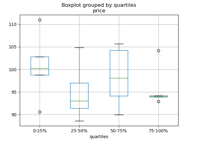
为分层变量的每个四分位数绘制箱型图
1
2
3
4
5
6
7
8
9
10
11
12
13
In [186 ]: df = pd.DataFrame( .....: {'stratifying_var' : np.random.uniform(0 , 100 , 20 ), .....: 'price' : np.random.normal(100 , 5 , 20 )}) .....: In [187 ]: df['quartiles' ] = pd.qcut( .....: df['stratifying_var' ], .....: 4 , .....: labels=['0-25%' , '25-50%' , '50-75%' , '75-100%' ]) .....: In [188 ]: df.boxplot(column='price' , by='quartiles' ) Out[188 ]: <matplotlib.axes._subplots.AxesSubplot at 0x7efff077f910 >
数据输入输出 SQL 与 HDF5 性能对比
CSV CSV 文档
read_csv 函数实战
把 DataFrame 追加到 CSV 文件
分块读取 CSV
分块读取指定的行
只读取 DataFrame 的前几列
读取不是 gzip 或 bz2 压缩(read_csv 可识别的内置压缩格式)的文件。本例在介绍如何读取 WinZip 压缩文件的同时,还介绍了在环境管理器里打开文件,并读取内容的通用操作方式。详见本链接
推断文件数据类型
处理出错数据
处理出错数据 II
用 Unix 时间戳读取 CSV,并转为本地时区
写入多行索引 CSV 时,不写入重复值
从多个文件读取数据,创建单个 DataFrame 最好的方式是先一个个读取单个文件,然后再把每个文件的内容存成列表,再用 pd.concat() 组合成一个 DataFrame:
1
2
3
4
5
6
7
8
In [189 ]: for i in range (3 ): .....: data = pd.DataFrame(np.random.randn(10 , 4 )) .....: data.to_csv('file_{}.csv' .format (i)) .....: In [190 ]: files = ['file_0.csv' , 'file_1.csv' , 'file_2.csv' ] In [191 ]: result = pd.concat([pd.read_csv(f) for f in files], ignore_index=True )
还可以用同样的方法读取所有匹配同一模式的文件,下面这个例子使用的是glob:
1
2
3
4
5
6
7
In [192 ]: import glob In [193 ]: import os In [194 ]: files = glob.glob('file_*.csv' ) In [195 ]: result = pd.concat([pd.read_csv(f) for f in files], ignore_index=True )
最后,这种方式也适用于 io 文档 介绍的其它 pd.read_* 函数。
解析多列里的日期组件 用一种格式解析多列的日期组件,速度更快。
1
2
3
4
5
6
7
8
9
10
11
12
13
14
15
16
17
18
19
20
21
In [196 ]: i = pd.date_range('20000101' , periods=10000 ) In [197 ]: df = pd.DataFrame({'year' : i.year, 'month' : i.month, 'day' : i.day}) In [198 ]: df.head() Out[198 ]: year month day 0 2000 1 1 1 2000 1 2 2 2000 1 3 3 2000 1 4 4 2000 1 5 In [199 ]: %timeit pd.to_datetime(df.year * 10000 + df.month * 100 + df.day, format ='%Y%m%d' ) .....: ds = df.apply(lambda x: "%04d%02d%02d" % (x['year' ], .....: x['month' ], x['day' ]), axis=1 ) .....: ds.head() .....: %timeit pd.to_datetime(ds) .....: 10.6 ms +- 698 us per loop (mean +- std. dev. of 7 runs, 100 loops each)3.21 ms +- 36.4 us per loop (mean +- std. dev. of 7 runs, 100 loops each)
跳过标题与数据之间的行 1 2 3 4 5 6 7 8 9 10 11 12 13 14 15 16 17 18 19 20 21 In [200 ]: data = """;;;; .....: ;;;; .....: ;;;; .....: ;;;; .....: ;;;; .....: ;;;; .....: ;;;; .....: ;;;; .....: ;;;; .....: ;;;; .....: date;Param1;Param2;Param4;Param5 .....: ;m²;°C;m²;m .....: ;;;; .....: 01.01.1990 00:00;1;1;2;3 .....: 01.01.1990 01:00;5;3;4;5 .....: 01.01.1990 02:00;9;5;6;7 .....: 01.01.1990 03:00;13;7;8;9 .....: 01.01.1990 04:00;17;9;10;11 .....: 01.01.1990 05:00;21;11;12;13 .....: """ .....:
选项 1:显式跳过行 1 2 3 4 5 6 7 8 9 10 11 12 13 14 In [201 ]: from io import StringIO In [202 ]: pd.read_csv(StringIO(data), sep=';' , skiprows=[11 , 12 ], .....: index_col=0 , parse_dates=True , header=10 ) .....: Out[202 ]: Param1 Param2 Param4 Param5 date 1990 -01-01 00 :00 :00 1 1 2 3 1990 -01-01 01:00 :00 5 3 4 5 1990 -01-01 02:00 :00 9 5 6 7 1990 -01-01 03:00 :00 13 7 8 9 1990 -01-01 04:00 :00 17 9 10 11 1990 -01-01 05:00 :00 21 11 12 13
选项 2:读取列名,然后再读取数据 1 2 3 4 5 6 7 8 9 10 11 12 13 14 15 16 17 In [203 ]: pd.read_csv(StringIO(data), sep=';' , header=10 , nrows=10 ).columns Out[203 ]: Index(['date' , 'Param1' , 'Param2' , 'Param4' , 'Param5' ], dtype='object' ) In [204 ]: columns = pd.read_csv(StringIO(data), sep=';' , header=10 , nrows=10 ).columns In [205 ]: pd.read_csv(StringIO(data), sep=';' , index_col=0 , .....: header=12 , parse_dates=True , names=columns) .....: Out[205 ]: Param1 Param2 Param4 Param5 date 1990 -01-01 00 :00 :00 1 1 2 3 1990 -01-01 01:00 :00 5 3 4 5 1990 -01-01 02:00 :00 9 5 6 7 1990 -01-01 03:00 :00 13 7 8 9 1990 -01-01 04:00 :00 17 9 10 11 1990 -01-01 05:00 :00 21 11 12 13
SQL SQL 文档
用 SQL 读取数据库
Excel Excel 文档
读取文件式句柄
用 XlsxWriter 修改输出格式
HTML 从不能处理默认请求 header 的服务器读取 HTML 表格
HDFStore HDFStores 文档
时间戳索引简单查询
用链式多表架构管理异构数据
在硬盘上合并数百万行的表格
避免多进程/线程存储数据出现不一致
按块对大规模数据存储去重的本质是递归还原操作。这里 介绍了一个函数,可以从 CSV 文件里按块提取数据,解析日期后,再按块存储。
按块读取 CSV 文件,并保存
追加到已存储的文件,且确保索引唯一
大规模数据工作流
读取一系列文件,追加时采用全局唯一索引
用低分组密度分组 HDFStore 文件
用高分组密度分组 HDFStore 文件
HDFStore 文件结构化查询
HDFStore 计数
HDFStore 异常解答
用字符串设置 min_itemsize
用 ptrepack 创建完全排序索引
把属性存至分组节点
1 2 3 4 5 6 7 8 9 10 11 In [206 ]: df = pd.DataFrame(np.random.randn(8 , 3 )) In [207 ]: store = pd.HDFStore('test.h5' ) In [208 ]: store.put('df' , df) In [209 ]: store.get_storer('df' ).attrs.my_attribute = {'A' : 10 } In [210 ]: store.get_storer('df' ).attrs.my_attribute Out[210 ]: {'A' : 10 }
二进制文件 读取 C 结构体数组组成的二进制文件,Pandas 支持 NumPy 记录数组。 比如说,名为 main.c 的文件包含下列 C 代码,并在 64 位机器上用 gcc main.c -std=gnu99 进行编译。
1 2 3 4 5 6 7 8 9 10 11 12 13 14 15 16 17 18 19 20 21 22 23 24 25 26 27 28 typedef struct _Data { int32_t count; double avg; float scale; } Data; int main(int argc, const char *argv[]){ size_t n = 10 ; Data d[n]; for (int i = 0 ; i < n; ++i) { d[i].count = i; d[i].avg = i + 1.0 ; d[i].scale = (float ) i + 2.0 f; } FILE *file = fopen("binary.dat" , "wb" ); fwrite(&d, sizeof(Data), n, file); fclose(file); return 0 ; }
下列 Python 代码读取二进制二建 binary.dat,并将之存为 pandas DataFrame,每个结构体的元素对应 DataFrame 里的列:
1 2 3 4 5 6 7 8 names = 'count' , 'avg' , 'scale' offsets = 0 , 8 , 16 formats = 'i4' , 'f8' , 'f4' dt = np.dtype({'names' : names, 'offsets' : offsets, 'formats' : formats}, align=True ) df = pd.DataFrame(np.fromfile('binary.dat' , dt))
::: tip 注意
不同机器上创建的文件因其架构不同,结构化元素的位移量也不同,原生二进制格式文件不能跨平台使用,因此不建议作为通用数据存储格式。建议用 Pandas IO 功能支持的 HDF5 或 msgpack 文件。
:::
计算 基于采样的时间序列数值整合
相关性 用 DataFrame.corr()where 可以实现这一功能:
1
2
3
4
5
6
7
8
9
10
11
12
13
14
In [211 ]: df = pd.DataFrame(np.random.random(size=(100 , 5 ))) In [212 ]: corr_mat = df.corr() In [213 ]: mask = np.tril(np.ones_like(corr_mat, dtype=np.bool ), k=-1 ) In [214 ]: corr_mat.where(mask) Out[214 ]: 0 1 2 3 4 0 NaN NaN NaN NaN NaN1 -0.018923 NaN NaN NaN NaN2 -0.076296 -0.012464 NaN NaN NaN3 -0.169941 -0.289416 0.076462 NaN NaN4 0.064326 0.018759 -0.084140 -0.079859 NaN
除了命名相关类型之外,DataFrame.corr 还接受回调,此处计算 DataFrame 对象的距离相关矩阵 。
1 2 3 4 5 6 7 8 9 10 11 12 13 14 15 16 17 18 19 20 21 22 23 24 25 26 27 28 In [215 ]: def distcorr (x, y ): .....: n = len (x) .....: a = np.zeros(shape=(n, n)) .....: b = np.zeros(shape=(n, n)) .....: for i in range (n): .....: for j in range (i + 1 , n): .....: a[i, j] = abs (x[i] - x[j]) .....: b[i, j] = abs (y[i] - y[j]) .....: a += a.T .....: b += b.T .....: a_bar = np.vstack([np.nanmean(a, axis=0 )] * n) .....: b_bar = np.vstack([np.nanmean(b, axis=0 )] * n) .....: A = a - a_bar - a_bar.T + np.full(shape=(n, n), fill_value=a_bar.mean()) .....: B = b - b_bar - b_bar.T + np.full(shape=(n, n), fill_value=b_bar.mean()) .....: cov_ab = np.sqrt(np.nansum(A * B)) / n .....: std_a = np.sqrt(np.sqrt(np.nansum(A**2 )) / n) .....: std_b = np.sqrt(np.sqrt(np.nansum(B**2 )) / n) .....: return cov_ab / std_a / std_b .....: In [216 ]: df = pd.DataFrame(np.random.normal(size=(100 , 3 ))) In [217 ]: df.corr(method=distcorr) Out[217 ]: 0 1 2 0 1.000000 0.199653 0.214871 1 0.199653 1.000000 0.195116 2 0.214871 0.195116 1.000000
时间差 时间差 文档。
使用时间差
1 2 3 4 5 6 7 8 9 10 11 12 13 14 15 16 17 18 19 20 21 22 23 24 25 26 27 28 29 30 31 32 33 34 35 36 37 38 39 40 41 42 43 44 45 In [218 ]: import datetime In [219 ]: s = pd.Series(pd.date_range('2012-1-1' , periods=3 , freq='D' )) In [220 ]: s - s.max () Out[220 ]: 0 -2 days1 -1 days2 0 daysdtype: timedelta64[ns] In [221 ]: s.max () - s Out[221 ]: 0 2 days1 1 days2 0 daysdtype: timedelta64[ns] In [222 ]: s - datetime.datetime(2011 , 1 , 1 , 3 , 5 ) Out[222 ]: 0 364 days 20 :55 :00 1 365 days 20 :55 :00 2 366 days 20 :55 :00 dtype: timedelta64[ns] In [223 ]: s + datetime.timedelta(minutes=5 ) Out[223 ]: 0 2012 -01-01 00 :05:00 1 2012 -01-02 00 :05:00 2 2012 -01-03 00 :05:00 dtype: datetime64[ns] In [224 ]: datetime.datetime(2011 , 1 , 1 , 3 , 5 ) - s Out[224 ]: 0 -365 days +03:05:00 1 -366 days +03:05:00 2 -367 days +03:05:00 dtype: timedelta64[ns] In [225 ]: datetime.timedelta(minutes=5 ) + s Out[225 ]: 0 2012 -01-01 00 :05:00 1 2012 -01-02 00 :05:00 2 2012 -01-03 00 :05:00 dtype: datetime64[ns]
日期加减
1 2 3 4 5 6 7 8 9 10 11 12 13 14 15 16 17 18 19 20 21 22 23 24 25 26 27 28 29 In [226 ]: deltas = pd.Series([datetime.timedelta(days=i) for i in range (3 )]) In [227 ]: df = pd.DataFrame({'A' : s, 'B' : deltas}) In [228 ]: df Out[228 ]: A B 0 2012 -01-01 0 days1 2012 -01-02 1 days2 2012 -01-03 2 daysIn [229 ]: df['New Dates' ] = df['A' ] + df['B' ] In [230 ]: df['Delta' ] = df['A' ] - df['New Dates' ] In [231 ]: df Out[231 ]: A B New Dates Delta 0 2012 -01-01 0 days 2012 -01-01 0 days1 2012 -01-02 1 days 2012 -01-03 -1 days2 2012 -01-03 2 days 2012 -01-05 -2 daysIn [232 ]: df.dtypes Out[232 ]: A datetime64[ns] B timedelta64[ns] New Dates datetime64[ns] Delta timedelta64[ns] dtype: object
其它示例
与 datetime 类似,用 np.nan 可以把值设为 NaT。
1 2 3 4 5 6 7 8 9 10 11 12 13 14 15 16 17 In [233 ]: y = s - s.shift() In [234 ]: y Out[234 ]: 0 NaT1 1 days2 1 daysdtype: timedelta64[ns] In [235 ]: y[1 ] = np.nan In [236 ]: y Out[236 ]: 0 NaT1 NaT2 1 daysdtype: timedelta64[ns]
轴别名 设置全局轴别名,可以定义以下两个函数:
1 2 3 4 5 6 7 8 9 10 11 12 13 14 15 16 17 18 19 20 21 22 23 24 In [237 ]: def set_axis_alias (cls, axis, alias ): .....: if axis not in cls._AXIS_NUMBERS: .....: raise Exception("invalid axis [%s] for alias [%s]" % (axis, alias)) .....: cls._AXIS_ALIASES[alias] = axis .....: In [238 ]: def clear_axis_alias (cls, axis, alias ): .....: if axis not in cls._AXIS_NUMBERS: .....: raise Exception("invalid axis [%s] for alias [%s]" % (axis, alias)) .....: cls._AXIS_ALIASES.pop(alias, None ) .....: In [239 ]: set_axis_alias(pd.DataFrame, 'columns' , 'myaxis2' ) In [240 ]: df2 = pd.DataFrame(np.random.randn(3 , 2 ), columns=['c1' , 'c2' ], .....: index=['i1' , 'i2' , 'i3' ]) .....: In [241 ]: df2.sum (axis='myaxis2' ) Out[241 ]: i1 -0.461013 i2 2.040016 i3 0.904681 dtype: float64 In [242 ]: clear_axis_alias(pd.DataFrame, 'columns' , 'myaxis2' )
创建示例数据 类似 R 的 expand.grid() 函数,用不同类型的值组生成 DataFrame,需要创建键是列名,值是数据值列表的字典:
1 2 3 4 5 6 7 8 9 10 11 12 13 14 15 16 17 18 19 20 21 22 23 24 25 In [243 ]: def expand_grid (data_dict ): .....: rows = itertools.product(*data_dict.values()) .....: return pd.DataFrame.from_records(rows, columns=data_dict.keys()) .....: In [244 ]: df = expand_grid({'height' : [60 , 70 ], .....: 'weight' : [100 , 140 , 180 ], .....: 'sex' : ['Male' , 'Female' ]}) .....: In [245 ]: df Out[245 ]: height weight sex 0 60 100 Male1 60 100 Female2 60 140 Male3 60 140 Female4 60 180 Male5 60 180 Female6 70 100 Male7 70 100 Female8 70 140 Male9 70 140 Female10 70 180 Male11 70 180 Female