
3_Regression demo(Adagrad)
Regression:linear model
这里用的是 Adagrad ,接下来的课程会再细讲,这里只是想显示 gradient descent 实作起来没有想像的那么简单,还有很多小技巧要注意
这里采用最简单的linear model:y_data=b+w*x_data
我们要用gradient descent把b和w找出来
当然这个问题有closed-form solution,这个b和w有更简单的方法可以找出来;那我们假装不知道这件事,我们练习用gradient descent把b和w找出来
数据准备:
1 | # 假设x_data和y_data都有10笔,分别代表宝可梦进化前后的cp值 |
计算梯度微分的函数getGrad()
1 | # 计算梯度微分的函数getGrad() |
1、自己写的版本
当两个微分值b_grad和w_grad都为0时,gradient descent停止,b和w的值就是我们要找的最终参数
1 | # 这是我自己写的版本,事实证明结果很糟糕。。。 |
the function will be y_data=-inf+nan*x_data
the average error is nan
上面的数据输出处于隐藏状态,点击即可显示
2、这里使用李宏毅老师的demo尝试
引入需要的库
1 | import matplotlib |
准备好b、w、loss的图像数据
1 | # 生成一组b和w的数据图,方便给gradient descent的过程做标记 |
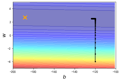
规定迭代次数和learning rate,进行第一次尝试
距离最优解还有一段距离
1 | # y_data = b + w * x_data |
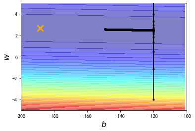
把learning rate增大10倍尝试
发现经过100000次的update以后,我们的参数相比之前与最终目标更接近了,但是这里有一个剧烈的震荡现象发生
1 | # 上图中,gradient descent最终停止的地方里最优解还差很远, |
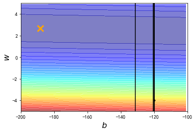
把learning rate再增大10倍
发现此时learning rate太大了,参数一update,就远远超出图中标注的范围了
所以我们会发现一个很严重的问题,如果learning rate变小一点,他距离最佳解还是会具有一段距离;但是如果learning rate放大,它就会直接超出范围了
1 | # 上图中,gradient descent最终停止的地方里最优解还是有一点远, |
这个问题明明很简单,可是只有两个参数b和w,gradient descent搞半天都搞不定,那以后做neural network有数百万个参数的时候,要怎么办呢
这个就是一室不治何以国家为的概念
解决方案:Adagrad
我们给b和w订制化的learning rate,让它们两个的learning rate不一样
1 | # 这里给b和w不同的learning rate |
the function will be y_data=-188.3668387495323+2.6692640713379903*x_data
error 0 is: 73.84441736270833
error 1 is: 67.4980970060185
error 2 is: 68.15177664932844
error 3 is: 28.8291759825683
error 4 is: 13.113158627146447
error 5 is: 148.63523696608252
error 6 is: 96.43143001996799
error 7 is: 94.21099446925288
error 8 is: 140.84008808876973
error 9 is: 161.7928115187101
the average error is 89.33471866905532
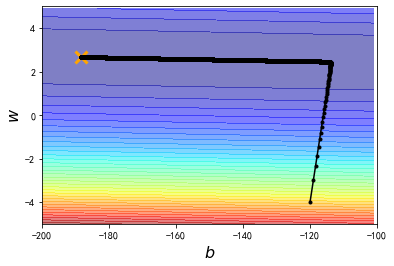
有了新的learning rate以后,从初始值到终点,我们在100000次iteration之内就可以顺利地完成了
本博客所有文章除特别声明外,均采用 CC BY-NC-SA 4.0 许可协议。转载请注明来源 Estom的博客!
相关推荐
2020-10-13
8_Deep Learning
Deep LearningUps and downs of Deep Learning 1958:Perceptron(linear model),感知机的提出 和Logistic Regression类似,只是少了sigmoid的部分 1969:Perceptron has limitation,from MIT 1980s:Multi-layer Perceptron,多层感知机 和今天的DNN很像 1986:Backpropagation,反向传播 Hinton propose的Backpropagation 存在problem:通常超过3个layer的neural network,就train不出好的结果 1989: 1 hidden layer is “good enough”,why deep? 有人提出一个理论:只要neural network有一个hidden layer,它就可以model出任何的function,所以根本没有必要叠加很多个hidden layer,所以Multi-layer Perceptron的方法又坏掉了,这段时间Multi-l...

2020-10-13
24_Transfer Learning
Transfer Learning 迁移学习,主要介绍共享layer的方法以及属性降维对比的方法 Introduction迁移学习,transfer learning,旨在利用一些不直接相关的数据对完成目标任务做出贡献 not directly related以猫狗识别为例,解释“不直接相关”的含义: input domain是类似的,但task是无关的 比如输入都是动物的图像,但这些data是属于另一组有关大象和老虎识别的task input domain是不同的,但task是一样的 比如task同样是做猫狗识别,但输入的是卡通类型的图像 compare with real life事实上,我们在日常生活中经常会使用迁移学习,比如我们会把漫画家的生活自动迁移类比到研究生的生活 overview迁移学习是很多方法的集合,这里介绍一些概念: Target Data:和task直接相关的data Source Data:和task没有直接关系的data 按照labeled data和unlabeled data又可以划分为四种: Case 1这里ta...

2021-08-01
《呼吸》
《商人和炼金术师之门》也许因为在做“科幻世界的电话”主题的分享,感觉电话与门有异曲同工之妙。主人公讲述了三位商人与一个炼金术师巴沙拉特的门的故事。 巴沙拉特展示了一种可以在过去和未来之间穿梭的神奇的年门,通过一个金属环的穿梭实验,展示了从一端到另一端会存在时间差。 第一个故事中,一个叫哈桑的绳匠,在二十年后的自己的指引下,躲过劫难,发现了一箱金子,然后发财,在二十年后成为了一个富豪。“仗势未来,横行现在的人,也许在第一次使用你年门的饿时候,就会发现他年长的自己早已亡故”。“忏悔和赎罪可以抹掉过去的罪孽”。“未来也是一样的,在这方面,它和过去没有区别”。故事没有着眼于未来与现在的矛盾,到底是先挖出箱子还是未来的人先知道箱子就在那里,无从得知。 第二个故事中,一个叫阿吉布的织工,发现二十年后的自己依旧穷困潦倒,却在床头存有一箱金币。于是从二十年后自己那里偷走了一箱金币,因此与爱慕的女人生活在一起,但是妻子却被强盗掳走,金币全都做了赎金。于是他开始一点点攒着金币,放在床头的箱子里,等着有朝一日,年轻的自己来偷走攒下的金币。同样他的妻子也回到过去,教会了他未来才掌握的、展示给妻子的东西。...

2020-09-26
date_index_formatter2
日期索引格式化程序在绘制每日数据时,频繁的请求是绘制忽略跳过的数据,例如,周末没有额外的空格。这在金融时间序列中尤为常见,因为您可能拥有M-F而非Sat,Sun的数据,并且您不需要x轴上的间隙。方法是简单地使用xdata的整数索引和自定义刻度Formatter来获取给定索引的适当日期字符串。 输出: 1loading /home/tcaswell/mc3/envs/dd37/lib/python3.7/site-packages/matplotlib/mpl-data/sample_data/msft.csv 12345678910111213141516171819202122232425262728293031323334import numpy as npimport matplotlib.pyplot as pltimport matplotlib.cbook as cbookfrom matplotlib.dates import bytespdate2num, num2datefrom matplotlib.ticker import Formatterdataf...
2020-09-24
7并发执行
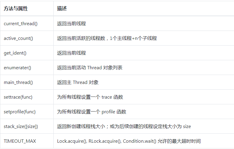
参考文献 7.1 基于线程的并发执行多线程实现方法和属性 theading模块包含以下的类: Thread: 基本线程类 Lock:互斥锁 RLock:可重入锁,使单一进程再次获得已持有的锁(递归锁) Condition:条件锁,使得一个线程等待另一个线程满足特定条件,比如改变状态或某个值。 Semaphore:信号锁,为线程间共享的有限资源提供一个”计数器”,如果没有可用资源则会被阻塞。 Event:事件锁,任意数量的线程等待某个事件的发生,在该事件发生后所有线程被激活。 Timer:一种计时器 Barrier:Python3.2新增的“阻碍”类,必须达到指定数量的线程后才可以继续执行。 面向对象实现方法123456789101112import threadingclass MyThread(threading.Thread): def __init__(self, thread_name): super(MyThread, self).__init__(name = thread_name) # 重写run()方法 def run(se...

2021-12-24
mpstat
mpstat显示各个可用CPU的状态 补充说明mpstat命令 指令主要用于多CPU环境下,它显示各个可用CPU的状态系你想。这些信息存放在/proc/stat文件中。在多CPUs系统里,其不但能查看所有CPU的平均状况信息,而且能够查看特定CPU的信息。 语法1mpstat(选项)(参数) 选项1-P:指定CPU编号。 参数 间隔时间:每次报告的间隔时间(秒); 次数:显示报告的次数。 实例当mpstat不带参数时,输出为从系统启动以来的平均值。 1234mpstatLinux 2.6.9-5.31AXsmp (builder.redflag-linux.com) 12/16/200509:38:46 AM CPU %user %nice %system %iowait %irq %soft %idle intr/s09:38:48 AM all 23.28 0.00 1.75 0.50 0.00 0.00 74.47 1018.59 每2秒产生了2个处理器的统计数据报告: 下面的命令可以每2秒产生了2个处理器的统计数据报告,一共产生三个interval 的...


