
plot_lasso_model_selection
Lasso模型选择:交叉验证 / AIC / BIC
本示例利用Akaike信息判据(AIC)、Bayes信息判据(BIC)和交叉验证,来筛选Lasso回归的正则化项参数alpha的最优值。
通过LassoLarsIC得到的结果,是基于AIC/BIC判据的。
这种基于信息判据(AIC/BIC)的模型选择非常快,但它依赖于对自由度的正确估计。该方式的假设模型必需是正确, 而且是对大样本(渐近结果)进行推导,即,数据实际上是由该模型生成的。当问题的背景条件很差时(特征数大于样本数),该模型选择方式会崩溃。
对于交叉验证,我们使用20-fold的2种算法来计算Lasso路径:LassoCV类实现的坐标下降和LassoLarsCV类实现的最小角度回归(Lars)。这两种算法给出的结果大致相同,但它们在执行速度和数值误差来源方面有所不同。
Lars仅为路径中的每个拐点计算路径解决方案。因此,当只有很少的弯折时,也就是很少的特征或样本时,它是非常有效的。此外,它能够计算完整的路径,而不需要设置任何元参数。与之相反,坐标下降算法计算预先指定的网格上的路径点(本示例中我们使用缺省值)。因此,如果网格点的数量小于路径中的拐点的数量,则效率更高。如果特征数量非常大,并且有足够的样本来选择大量特征,那么这种策略就非常有趣。在数值误差方面,Lars会因变量间的高相关度而积累更多的误差,而坐标下降算法只会采样网格上路径。
注意观察alpha的最优值是如何随着每个fold而变化。这是为什么当估交叉验证选择参数的方法的性能时,需要使用嵌套交叉验证的原因:这种参数的选择对于不可见数据可能不是最优的。
1 | import time |
1 | # 这样做是为了避免在np.log10时除零 |
1 | # 将最小角度回归得到的数据标准化,以便进行比较 |
1 | # LassoLarsIC: 用BIC/AIC判据进行最小角度回归 |
1 | def plot_ic_criterion(model, name, color): |
Text(0.5, 1.0, '模型选择的信息判据 (训练时间:0.024s)')

1 | # LassoCV: 坐标下降 |
(2300, 3800)

1 | # LassoLarsCV: 最小角度回归法 |
Computing regularization path using the Lars lasso...

本博客所有文章除特别声明外,均采用 CC BY-NC-SA 4.0 许可协议。转载请注明来源 Estom的博客!
相关推荐

2020-07-08
04 属性配置文件
属性配置文件 bean配置文件:spring配置bean的文件。 java配置文件,通过@Configuration加载 原生配置文件,xml定义的配置文件 属性配置文件:spring配置key-value的文件 1 properties配置文件properties默认配置文件用于配置容器端口名、数据库链接信息、日志级别。pom是项目编程的配置,properties是软件部署的配置。 移除特殊字符、全小写。在环境变量中通过小写转换与.替换_来映射配置文件中的内容,比如:环境变量SPRING_JPA_DATABASEPLATFORM=mysql的配置会产生与在配置文件中设置spring.jpa.databaseplatform=mysql一样的效果。 1src/main/resources/application.properties 1234environments.dev.url=http://dev.bar.comenvironments.dev.name=Developer Setupenvironments.prod.url=http://...
2021-03-20
19
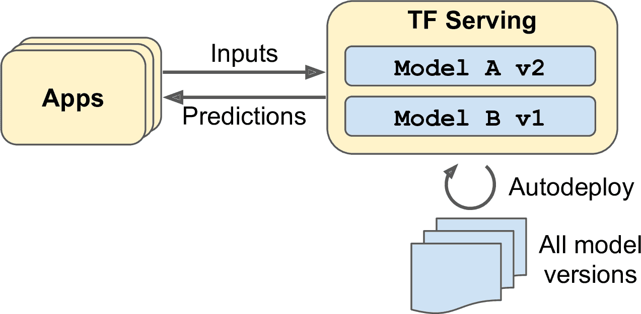
十九、规模化训练和部署 TensorFlow 模型 译者:@SeanCheney 有了能做出惊人预测的模型之后,要做什么呢?当然是部署生产了。这只要用模型运行一批数据就成,可能需要写一个脚本让模型每夜都跑着。但是,现实通常会更复杂。系统基础组件都可能需要这个模型用于实时数据,这种情况需要将模型包装成网络服务:这样的话,任何组件都可以通过 REST API 询问模型。随着时间的推移,你需要用新数据重新训练模型,更新生产版本。必须处理好模型版本,平稳地过渡到新版本,碰到问题的话需要回滚,也许要并行运行多个版本做 AB 测试。如果产品很成功,你的服务可能每秒会有大量查询,系统必须提升负载能力。提升负载能力的方法之一,是使用 TF Serving,通过自己的硬件或通过云服务,比如 Google Cloud API 平台。TF Serving 能高效服务化模型,优雅处理模型过渡,等等。如果使用云平台,还能获得其它功能,比如强大的监督工具。 另外,如果有很多训练数据和计算密集型模型,则训练时间可能很长。如果产品需要快速迭代,这么长的训练时间是不可接受的(例如,新闻推荐系统总是推荐上个星期的...
2020-09-27
8.回归
第8章 预测数值型数据: 回归回归(Regression) 概述我们前边提到的分类的目标变量是标称型数据,而回归则是对连续型的数据做出处理,回归的目的是预测数值型数据的目标值。 回归 场景回归的目的是预测数值型的目标值。最直接的办法是依据输入写出一个目标值的计算公式。 假如你想要预测兰博基尼跑车的功率大小,可能会这样计算: HorsePower = 0.0015 * annualSalary - 0.99 * hoursListeningToPublicRadio 这就是所谓的 回归方程(regression equation),其中的 0.0015 和 -0.99 称作 回归系数(regression weights),求这些回归系数的过程就是回归。一旦有了这些回归系数,再给定输入,做预测就非常容易了。具体的做法是用回归系数乘以输入值,再将结果全部加在一起,就得到了预测值。我们这里所说的,回归系数是一个向量,输入也是向量,这些运算也就是求出二者的内积。 说到回归,一般都是指 线性回归(linear regression)。线性回归意味着可以将输入项分别乘以一些常量,再...
2021-03-20
20
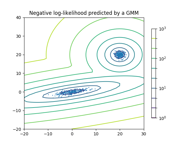
2.1. 高斯混合模型校验者: @why2lyj @Shao Y. @Loopy @barrycg翻译者: @glassy sklearn.mixture 是一个应用高斯混合模型进行非监督学习的包(支持 diagonal,spherical,tied,full 四种协方差矩阵), (注:diagonal 指每个分量有各自独立的对角协方差矩阵, spherical 指每个分量有各自独立的方差(再注:spherical是一种特殊的 diagonal, 对角的元素相等), tied 指所有分量共享一个标准协方差矩阵, full 指每个分量有各自独立的标准协方差矩阵),它可以对数据进行抽样,并且根据数据来估计模型。同时该包也支持由用户来决定模型内混合的分量数量。 (译注:在高斯混合模型中,我们将每一个高斯分布称为一个分量,即 component) 二分量高斯混合模型: 数据点,以及模型的等概率线。 高斯混合模型是一个假设所有的数据点都是生成于有限个带有未知参数的高斯分布所混合的概率模型。 我们可以将这种混合模型看作...

2021-12-24
vgscan
vgscan扫描并显示系统中的卷组 补充说明vgscan命令 查找系统中存在的LVM卷组,并显示找到的卷组列表。vgscan命令仅显示找到的卷组的名称和LVM元数据类型,要得到卷组的详细信息需要使用vgdisplay命令。 语法1vgscan(选项) 选项12-d:调试模式;--ignorerlockingfailure:忽略锁定失败的错误。 实例使用vgscan命令扫描系统中所有的卷组。在命令行中输入下面的命令: 1[root@localhost ~]# vgscan #扫描并显示LVM卷组列表 输出信息如下: 12Found volume group "vg2000" using metadata type lvm2 Found volume group "vg1000" using metadata type lvm2 说明:本例中,vgscan指令找到了两个LVM2卷组”vg1000”和”vg2000”。

2021-03-22
42 分布式数据并行
分布式数据并行入门 原文:https://pytorch.org/tutorials/intermediate/ddp_tutorial.html 作者:Shen Li 编辑:Joe Zhu 先决条件: PyTorch 分布式概述 DistributedDataParallel API 文档 DistributedDataParallel注意事项 DistributedDataParallel(DDP)在模块级别实现可在多台计算机上运行的数据并行性。 使用 DDP 的应用应产生多个进程,并为每个进程创建一个 DDP 实例。 DDP 在torch.distributed包中使用集体通信来同步梯度和缓冲区。 更具体地说,DDP 为model.parameters()给定的每个参数注册一个 Autograd 挂钩,当在后向传递中计算相应的梯度时,挂钩将触发。 然后,DDP 使用该信号触发跨进程的梯度同步。 有关更多详细信息,请参考 DDP 设计说明。 推荐的使用 DDP 的方法是为每个模型副本生成一个进程,其中一个模型副本可以跨越多个设备。 DDP 进程可以放在同一台计算机上,也...


