57

把它们放在一起

校验者:
        @片刻
翻译者:
        @X

模型管道化

我们已经知道一些模型可以做数据转换，一些模型可以用来预测变量。我们可以建立一个组合模型同时完成以上工作:

import numpy as np
import matplotlib.pyplot as plt
import pandas as pd

from sklearn import datasets
from sklearn.decomposition import PCA
from sklearn.linear_model import SGDClassifier
from sklearn.pipeline import Pipeline
from sklearn.model_selection import GridSearchCV


# Define a pipeline to search for the best combination of PCA truncation
# and classifier regularization.
logistic = SGDClassifier(loss='log', penalty='l2', early_stopping=True,
                         max_iter=10000, tol=1e-5, random_state=0)
pca = PCA()
pipe = Pipeline(steps=[('pca', pca), ('logistic', logistic)])

digits = datasets.load_digits()
X_digits = digits.data
y_digits = digits.target

# Parameters of pipelines can be set using ‘__’ separated parameter names:
param_grid = {
    'pca__n_components': [5, 20, 30, 40, 50, 64],
    'logistic__alpha': np.logspace(-4, 4, 5),
}
search = GridSearchCV(pipe, param_grid, iid=False, cv=5)
search.fit(X_digits, y_digits)
print("Best parameter (CV score=%0.3f):" % search.best_score_)
print(search.best_params_)

# Plot the PCA spectrum
pca.fit(X_digits)

fig, (ax0, ax1) = plt.subplots(nrows=2, sharex=True, figsize=(6, 6))
ax0.plot(pca.explained_variance_ratio_, linewidth=2)
ax0.set_ylabel('PCA explained variance')

ax0.axvline(search.best_estimator_.named_steps['pca'].n_components,
            linestyle=':', label='n_components chosen')

用特征面进行人脸识别

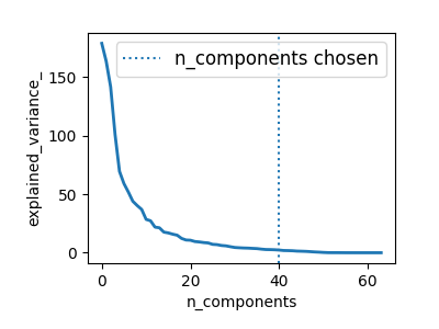
该实例用到的数据集来自 LFW_(Labeled Faces in the Wild)。数据已经进行了初步预处理

http://vis-www.cs.umass.edu/lfw/lfw-funneled.tgz (233MB)

"""
===================================================
Faces recognition example using eigenfaces and SVMs
===================================================

The dataset used in this example is a preprocessed excerpt of the
"Labeled Faces in the Wild", aka LFW_:

  http://vis-www.cs.umass.edu/lfw/lfw-funneled.tgz (233MB)

.. _LFW: http://vis-www.cs.umass.edu/lfw/

Expected results for the top 5 most represented people in the dataset:

================== ============ ======= ========== =======
                   precision    recall  f1-score   support
================== ============ ======= ========== =======
     Ariel Sharon       0.67      0.92      0.77        13
     Colin Powell       0.75      0.78      0.76        60
  Donald Rumsfeld       0.78      0.67      0.72        27
    George W Bush       0.86      0.86      0.86       146
Gerhard Schroeder       0.76      0.76      0.76        25
      Hugo Chavez       0.67      0.67      0.67        15
       Tony Blair       0.81      0.69      0.75        36

      avg / total       0.80      0.80      0.80       322
================== ============ ======= ========== =======

"""
from time import time
import logging
import matplotlib.pyplot as plt

from sklearn.model_selection import train_test_split
from sklearn.model_selection import GridSearchCV
from sklearn.datasets import fetch_lfw_people
from sklearn.metrics import classification_report
from sklearn.metrics import confusion_matrix
from sklearn.decomposition import PCA
from sklearn.svm import SVC


print(__doc__)

# Display progress logs on stdout
logging.basicConfig(level=logging.INFO, format='%(asctime)s %(message)s')


# #############################################################################
# Download the data, if not already on disk and load it as numpy arrays

lfw_people = fetch_lfw_people(min_faces_per_person=70, resize=0.4)

# introspect the images arrays to find the shapes (for plotting)
n_samples, h, w = lfw_people.images.shape

# for machine learning we use the 2 data directly (as relative pixel
# positions info is ignored by this model)
X = lfw_people.data
n_features = X.shape[1]

# the label to predict is the id of the person
y = lfw_people.target
target_names = lfw_people.target_names
n_classes = target_names.shape[0]

print("Total dataset size:")
print("n_samples: %d" % n_samples)
print("n_features: %d" % n_features)
print("n_classes: %d" % n_classes)


# #############################################################################
# Split into a training set and a test set using a stratified k fold

# split into a training and testing set
X_train, X_test, y_train, y_test = train_test_split(
    X, y, test_size=0.25, random_state=42)


# #############################################################################
# Compute a PCA (eigenfaces) on the face dataset (treated as unlabeled
# dataset): unsupervised feature extraction / dimensionality reduction
n_components = 150

print("Extracting the top %d eigenfaces from %d faces"
      % (n_components, X_train.shape[0]))
t0 = time()
pca = PCA(n_components=n_components, svd_solver='randomized',
          whiten=True).fit(X_train)
print("done in %0.3fs" % (time() - t0))

eigenfaces = pca.components_.reshape((n_components, h, w))

print("Projecting the input data on the eigenfaces orthonormal basis")
t0 = time()
X_train_pca = pca.transform(X_train)
X_test_pca = pca.transform(X_test)
print("done in %0.3fs" % (time() - t0))


# #############################################################################
# Train a SVM classification model

print("Fitting the classifier to the training set")
t0 = time()
param_grid = {'C': [1e3, 5e3, 1e4, 5e4, 1e5],
              'gamma': [0.0001, 0.0005, 0.001, 0.005, 0.01, 0.1], }
clf = GridSearchCV(SVC(kernel='rbf', class_weight='balanced'),
                   param_grid, cv=5, iid=False)
clf = clf.fit(X_train_pca, y_train)
print("done in %0.3fs" % (time() - t0))
print("Best estimator found by grid search:")
print(clf.best_estimator_)


# #############################################################################
# Quantitative evaluation of the model quality on the test set

print("Predicting people's names on the test set")
t0 = time()
y_pred = clf.predict(X_test_pca)
print("done in %0.3fs" % (time() - t0))

print(classification_report(y_test, y_pred, target_names=target_names))
print(confusion_matrix(y_test, y_pred, labels=range(n_classes)))


# #############################################################################
# Qualitative evaluation of the predictions using matplotlib

def plot_gallery(images, titles, h, w, n_row=3, n_col=4):
    """Helper function to plot a gallery of portraits"""
    plt.figure(figsize=(1.8 * n_col, 2.4 * n_row))
    plt.subplots_adjust(bottom=0, left=.01, right=.99, top=.90, hspace=.35)
    for i in range(n_row * n_col):
        plt.subplot(n_row, n_col, i + 1)
        plt.imshow(images[i].reshape((h, w)), cmap=plt.cm.gray)
        plt.title(titles[i], size=12)
        plt.xticks(())
        plt.yticks(())


# plot the result of the prediction on a portion of the test set

def title(y_pred, y_test, target_names, i):
    pred_name = target_names[y_pred[i]].rsplit(' ', 1)[-1]
    true_name = target_names[y_test[i]].rsplit(' ', 1)[-1]
    return 'predicted: %s\ntrue:      %s' % (pred_name, true_name)

prediction_titles = [title(y_pred, y_test, target_names, i)
                     for i in range(y_pred.shape[0])]

plot_gallery(X_test, prediction_titles, h, w)

# plot the gallery of the most significative eigenfaces

eigenface_titles = ["eigenface %d" % i for i in range(eigenfaces.shape[0])]
plot_gallery(eigenfaces, eigenface_titles, h, w)

plt.show()

Prediction	Eigenfaces

数据集中前5名最有代表性样本的预期结果:

                   precision    recall  f1-score   support

Gerhard_Schroeder       0.91      0.75      0.82        28
  Donald_Rumsfeld       0.84      0.82      0.83        33
       Tony_Blair       0.65      0.82      0.73        34
     Colin_Powell       0.78      0.88      0.83        58
    George_W_Bush       0.93      0.86      0.90       129

      avg / total       0.86      0.84      0.85       282

开放性问题: 股票市场结构

我们可以预测 Google 在特定时间段内的股价变动吗？

Learning a graph structure