26

5.4 – Batch Normalization 批标准化

批标准化通俗来说就是对每一层神经网络进行标准化 (normalize) 处理, 我们知道对输入数据进行标准化能让机器学习有效率地学习. 如果把每一层后看成这种接受输入数据的模式, 那我们何不 “批标准化” 所有的层呢? 具体而且清楚的解释请看到 我（原作者）制作的 什么批标准化 动画简介(推荐)（如下）.

那我们就看看下面的两个动图, 这就是在每层神经网络有无 batch normalization 的区别啦.

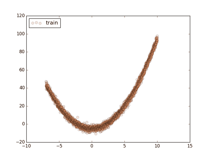
做点数据

自己做一些伪数据, 用来模拟真实情况. 而且 Batch Normalization (之后都简称BN) 还能有效的控制坏的参数初始化 (initialization), 比如说 ReLU  这种激励函数最怕所有的值都落在附属区间, 那我们就将所有的参数都水平移动一个 -0.2 ( bias_initialization = -0.2 , 来看看 BN 的实力.

import torch
from torch.autograd import Variable
from torch import nn
from torch.nn import init
import torch.utils.data as Data
import torch.nn.functional as F
import matplotlib.pyplot as plt
import numpy as np

# 超参数
N_SAMPLES = 2000
BATCH_SIZE = 64
EPOCH = 12
LR = 0.03
N_HIDDEN = 8
ACTIVATION = F.tanh     # 你可以换 relu 试试
B_INIT = -0.2   # 模拟不好的 参数初始化

# training data
x = np.linspace(-7, 10, N_SAMPLES)[:, np.newaxis]
noise = np.random.normal(0, 2, x.shape)
y = np.square(x) - 5   noise

# test data
test_x = np.linspace(-7, 10, 200)[:, np.newaxis]
noise = np.random.normal(0, 2, test_x.shape)
test_y = np.square(test_x) - 5   noise

train_x, train_y = torch.from_numpy(x).float(), torch.from_numpy(y).float()
test_x = Variable(torch.from_numpy(test_x).float(), volatile=True)  # volatile=True 不进行梯度计算
test_y = Variable(torch.from_numpy(test_y).float(), volatile=True)

train_dataset = Data.TensorDataset(data_tensor=train_x, target_tensor=train_y)
train_loader = Data.DataLoader(dataset=train_dataset, batch_size=BATCH_SIZE, shuffle=True, num_workers=2,)

# show data
plt.scatter(train_x.numpy(), train_y.numpy(), c=\'#FF9359\', s=50, alpha=0.2, label=\'train\')
plt.legend(loc=\'upper left\')
plt.show()

搭建神经网络

这里就教你如何构建带有 BN 的神经网络的. BN 其实可以看做是一个 layer ( BN layer ). 我们就像平时加层一样加 BN layer  就好了. 注意, 我还对输入数据进行了一个 BN 处理, 因为如果你把输入数据看出是 从前面一层来的输出数据, 我们同样也能对她进行 BN.

class Net(nn.Module):
    def __init__(self, batch_normalization=False):
        super(Net, self).__init__()
        self.do_bn = batch_normalization
        self.fcs = []   # 太多层了, 我们用 for loop 建立
        self.bns = []
        self.bn_input = nn.BatchNorm1d(1, momentum=0.5)   # 给 input 的 BN

        for i in range(N_HIDDEN):               # 建层
            input_size = 1 if i == 0 else 10
            fc = nn.Linear(input_size, 10)
            setattr(self, \'fc%i\' % i, fc)       # 注意! pytorch 一定要你将层信息变成 class 的属性! 我在这里花了2天时间发现了这个 bug
            self._set_init(fc)                  # 参数初始化
            self.fcs.append(fc)
            if self.do_bn:
                bn = nn.BatchNorm1d(10, momentum=0.5)
                setattr(self, \'bn%i\' % i, bn)   # 注意! pytorch 一定要你将层信息变成 class 的属性! 我在这里花了2天时间发现了这个 bug
                self.bns.append(bn)

        self.predict = nn.Linear(10, 1)         # output layer
        self._set_init(self.predict)            # 参数初始化

    def _set_init(self, layer):     # 参数初始化
        init.normal(layer.weight, mean=0., std=.1)
        init.constant(layer.bias, B_INIT)

    def forward(self, x):
        pre_activation = [x]
        if self.do_bn: x = self.bn_input(x)    # 判断是否要加 BN
        layer_input = [x]
        for i in range(N_HIDDEN):
            x = self.fcs[i](x)
            pre_activation.append(x)    # 为之后出图
            if self.do_bn: x = self.bns[i](x)  # 判断是否要加 BN
            x = ACTIVATION(x)
            layer_input.append(x)       # 为之后出图
        out = self.predict(x)
        return out, layer_input, pre_activation

# 建立两个 net, 一个有 BN, 一个没有
nets = [Net(batch_normalization=False), Net(batch_normalization=True)]

训练

训练的时候, 这两个神经网络分开训练. 训练的环境都一样.

opts = [torch.optim.Adam(net.parameters(), lr=LR) for net in nets]

loss_func = torch.nn.MSELoss()

losses = [[], []]  # 每个网络一个 list 来记录误差
for epoch in range(EPOCH):
    print(\'Epoch: \', epoch)
    for step, (b_x, b_y) in enumerate(train_loader):
        b_x, b_y = Variable(b_x), Variable(b_y)
        for net, opt in zip(nets, opts):     # 训练两个网络
            pred, _, _ = net(b_x)
            loss = loss_func(pred, b_y)
            opt.zero_grad()
            loss.backward()
            opt.step()    # 这也会训练 BN 里面的参数

画图

这个教程有几张图要画, 首先我们画训练时的动态图. 我单独定义了一个画动图的功能 plot_histogram() , 因为不是重点, 所以代码的具体细节请看我的 github,

f, axs = plt.subplots(4, N_HIDDEN 1, figsize=(10, 5))

def plot_histogram(l_in, l_in_bn, pre_ac, pre_ac_bn):
    ...

for epoch in range(EPOCH):
    layer_inputs, pre_acts = [], []
    for net, l in zip(nets, losses):
        # 一定要把 net 的设置成 eval 模式, eval下的 BN 参数会被固定
        net.eval()
        pred, layer_input, pre_act = net(test_x)
        l.append(loss_func(pred, test_y).data[0])
        layer_inputs.append(layer_input)
        pre_acts.append(pre_act)
        # 收集好信息后将 net 设置成 train 模式, 继续训练
        net.train()
    plot_histogram(*layer_inputs, *pre_acts)     # plot histogram

    # 后面接着之前 for loop 中的代码来
    for step, (b_x, b_y) in enumerate(train_loader):
    ...

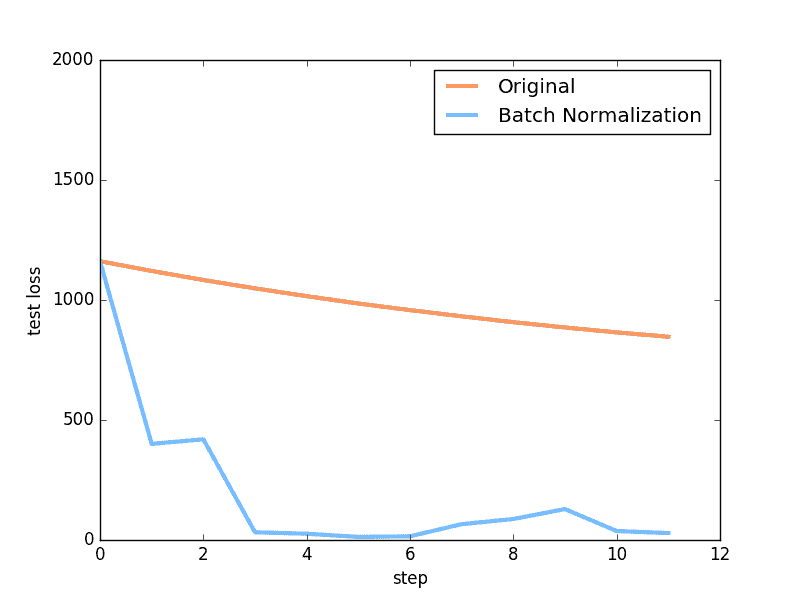
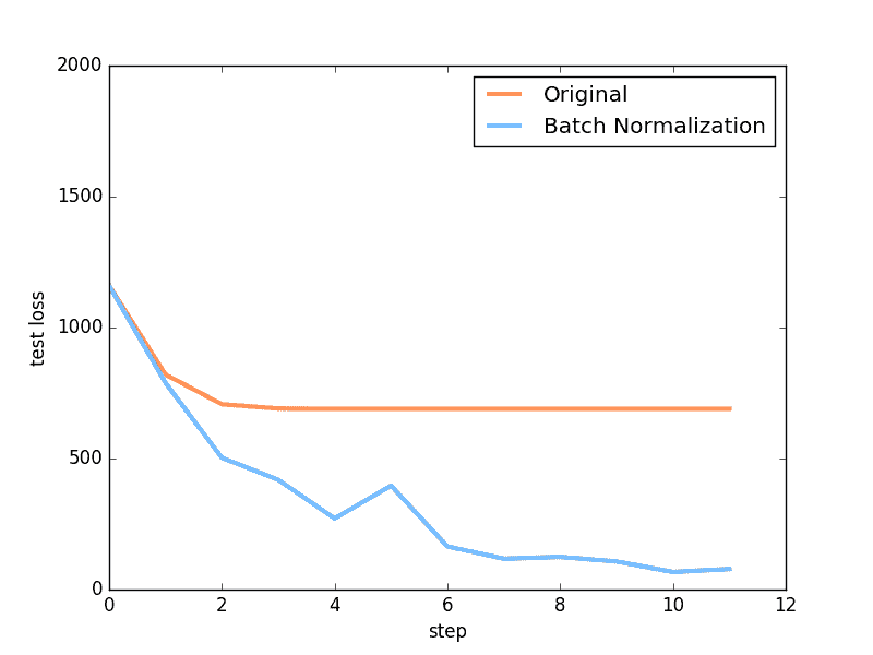
后面还有两张图, 一张是预测曲线, 一张是误差变化曲线, 具体代码不在这里呈现, 想知道如何画图的朋友, 请参考我的 github

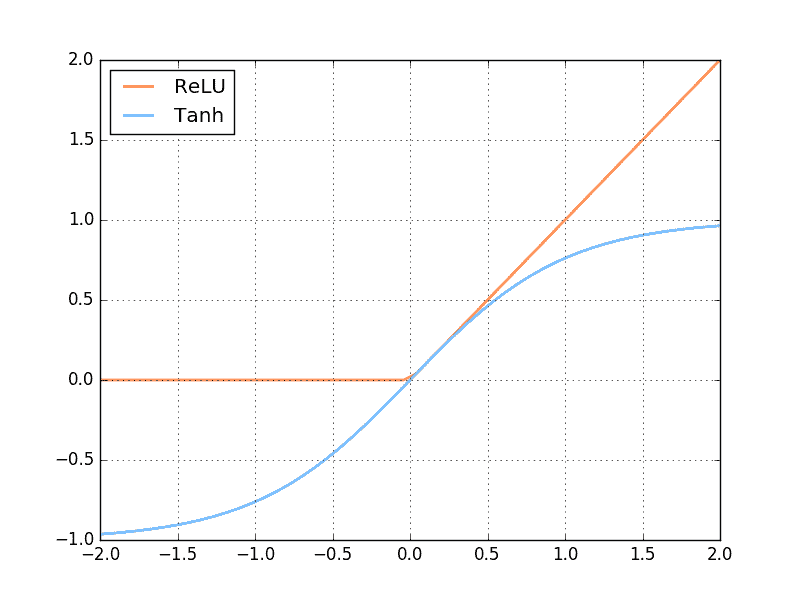
对比结果

首先来看看这次对比的两个激励函数是长什么样:

然后我们来对比使用不同激励函数的结果.

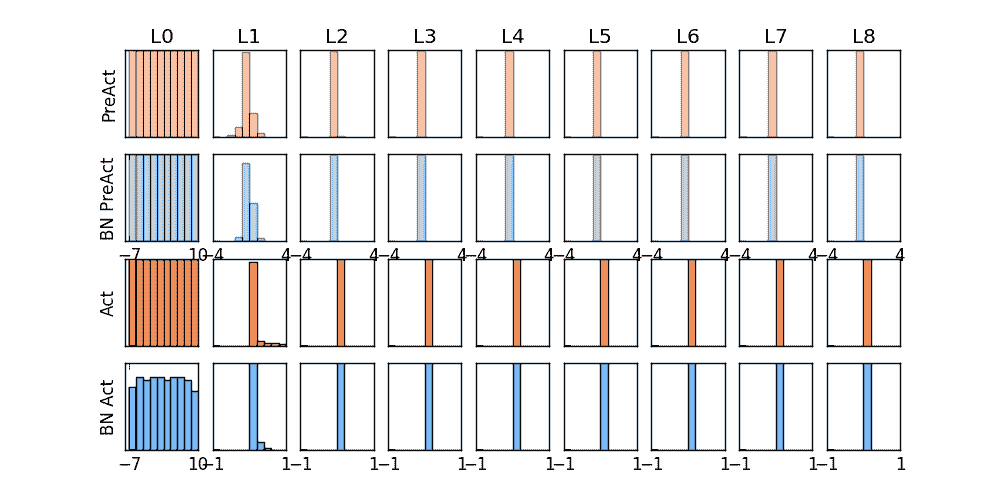
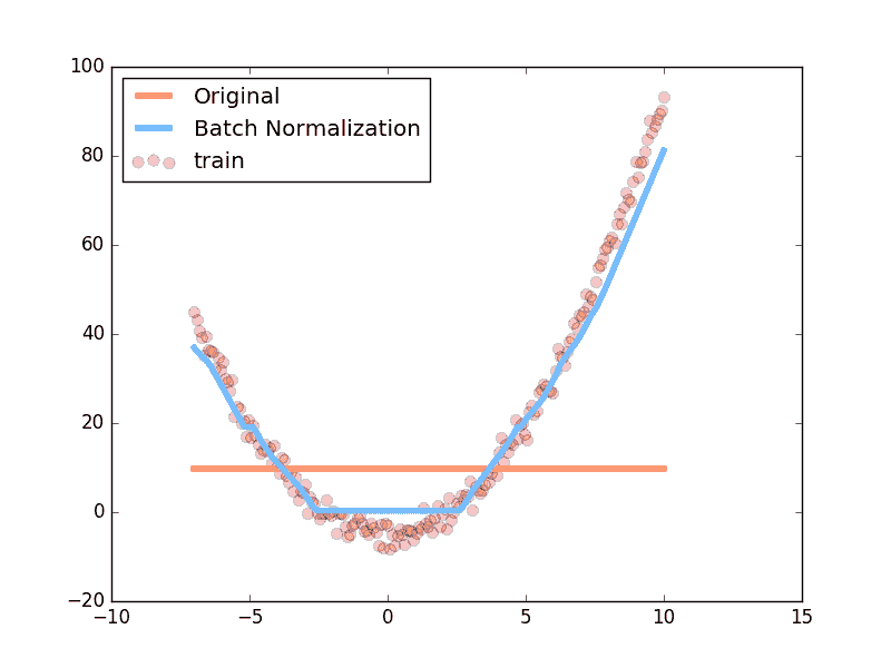
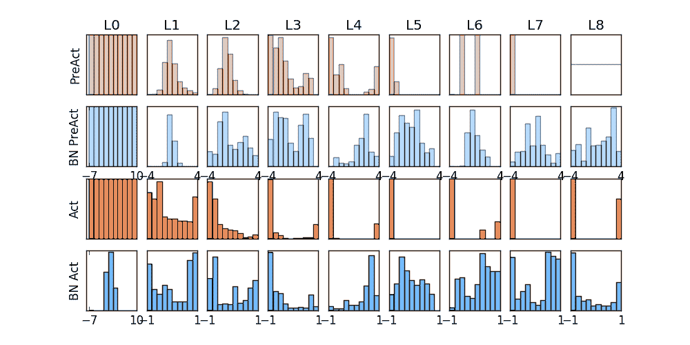
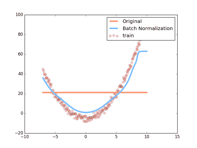
上面是使用 relu  激励函数的结果, 我们可以看到, 没有使用 BN 的误差要高, 线条不能拟合数据, 原因是我们有一个 “Bad initialization”, 初始 bias = -0.2 , 这一招, 让 relu  无法捕捉到在负数区间的输入值. 而有了 BN, 这就不成问题了.

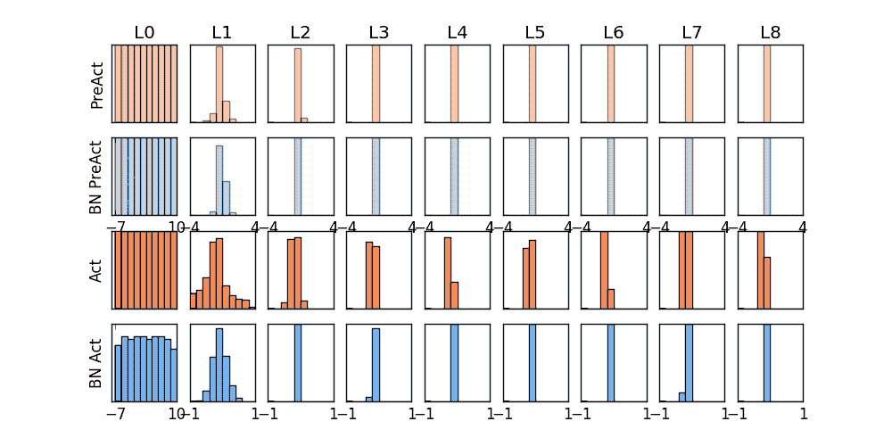
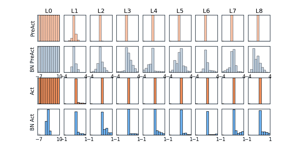
上面结果是使用 tanh  作为激励函数的结果, 可以看出, 不好的初始化, 让输入数据在激活前分散得非常离散, 而有了 BN, 数据都被收拢了. 收拢的数据再放入激励函数就能很好地利用激励函数的非线性. 而且可以看出没有 BN 的数据让激活后的结果都分布在 tanh  的两端, 而这两端的梯度又非常的小, 是的后面的误差都不能往前传, 导致神经网络死掉了.

所以这也就是在我 github 代码 中的每一步的意义啦.

文章来源：莫烦